Challenge

Project 2 Thermal modeling of battery pack

SSaurav Kumar Singha26 Oct 2022

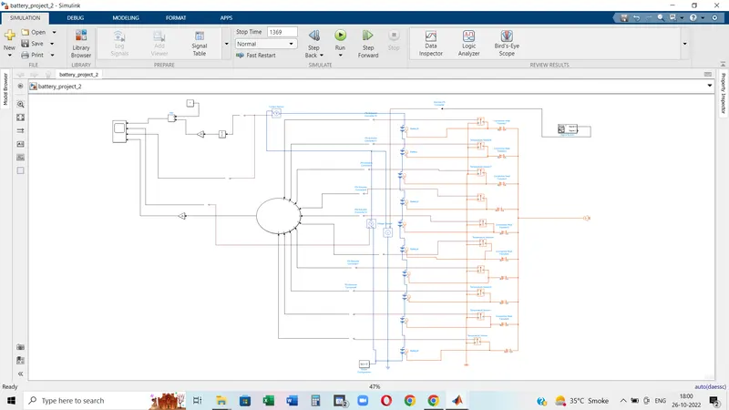
For a 10-cell series lithium-ion battery model, simulate the thermal effects and compare life cycle performance at various temperatures, charge & discharge rates using MATLAB :

Objective: Simulating Li-ion battery model to determine the thermal effects and life cycle performance at various temperatures, charge-discharge cycle

Model:

Used Blocks:

1. Battery:

The Battery block represents a simple battery model. The block has four modeling variants, accessible by right-clicking the block in your block diagram and then selecting the appropriate option from the context menu, under Simscape > Block choices:

Uninstrumented | No thermal port — A basic model that does not output battery charge level or simulates thermal effects. This modeling variant is the default.
Uninstrumented | Show thermal port — Model with exposed thermal port. This model does not measure the internal charge level of the battery.
Instrumented | No thermal port — Model with an exposed charge output port. This model does not simulate thermal effects.
Instrumented | Show thermal port — Model that lets you measure the internal charge level of the battery and simulate thermal effects. Both the thermal port and the charge output port are exposed.

If you select Infinite for the Battery charge capacity parameter, the block models the battery as a series resistor and a constant voltage source. If you select Finite for the Battery charge capacity parameter, the block models the battery as a series resistor and a charge-dependent voltage source. In the finite case, the voltage is a function of charge and has the following relationship:

V=V0(SOC1−β(1−SOC))

where:

SOC (state-of-charge) is the ratio of current charge to rated battery capacity.
V₀ is the voltage when the battery is fully charged at no load, as defined by the Nominal voltage, Vnom parameter.
β is a constant that is calculated so that the battery voltage is V1 when the charge is AH1. Specify the voltage V1 and ampere-hour rating AH1 using block parameters. AH1 is the charge when the no-load (open-circuit) voltage is V1, and V1 is less than the nominal voltage.

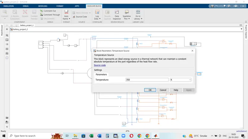
2. Temperature Source:

The Temperature Source block represents an ideal source of thermal energy that is powerful enough to maintain a specified temperature at its outlet regardless of the heat flow consumed by the system.
The source generates constant absolute temperature, defined by the Temperature parameter value.
Port: Thermal conserving port associated with the source outlet.

3. Convective Heat Transfer:

Convection is the transfer of heat from one place to another due to the movement of fluid. Although often discussed as a distinct method of heat transfer, convective heat transfer involves the combined processes of conduction and advection. Convection is usually the dominant form of heat transfer in liquids and gases.

The Convective Heat Transfer block represents a heat transfer by convection between two bodies by means of fluid motion. The transfer is governed by the Newton law of cooling and is described with the following equation:

Q=k·A·(TA−TB),

where

Q= Heat flow

k= Convection heat transfer coefficient

T_A, T_B=Temperatures of the bodies

A= Surface area

The block has the following ports:

A= Thermal conserving port associated with body A.

B= Thermal conserving port associated with body B.

4. Temperature Sensor:

The Temperature Sensor block represents an ideal temperature sensor, that is, a device that determines the temperature differential measured between two points without drawing any heat.
Connections A and B are thermal conserving ports that connect to the two points where the temperature is being monitored. Port T is a physical signal port that outputs the temperature differential value.
The block's positive direction is from port A to port B. The measured temperature is determined as T = T_A – T_B.
The block has the following ports:

A= Thermal conserving port associated with the sensor positive probe.

B= Thermal conserving port associated with the sensor negative probe.

T= Physical signal output port for temperature.

5. Controlled Current Source:

The Controlled Current Source block represents an ideal current source that is powerful enough to maintain the specified current through it regardless of the voltage across the source.
The output current is I = Is, where Is is the numerical value presented at the physical signal port.
The positive direction of the current flow is indicated by the arrow.
The block has one physical signal input port and two electrical conserving ports associated with its electrical terminals

6. Voltage Sensor:

The Voltage Sensor block represents an ideal voltage sensor, that is, a device that converts voltage measured between two points of an electrical circuit into a physical signal proportional to the voltage.
Connections + and – are electrical conserving ports through which the sensor is connected to the circuit. Connection V is a physical signal port that outputs the measurement result.

The block has the following ports:

+ :Electrical conserving port associated with the sensor positive terminal.
- : Electrical conserving port associated with the sensor negative terminal.
V : Physical signal output port for voltage.

7. Integration:

The Integrator block outputs the value of the integral of its input signal with respect to time.

Simulink^® treats the Integrator block as a dynamic system with one state. The block dynamics are given by:

x(t)=u(t)

y(t)=x(t)

x(t0)=x0

where:

u is the block input.
y is the block output.
x is the block state.
x₀ is the initial condition of x.

While these equations define an exact relationship in continuous time, Simulink uses numerical approximation methods to evaluate them with finite precision. Simulink can use several different numerical integration methods to compute the output of the block, each with advantages in particular applications. Use the Solver pane of the Configuration Parameters dialog box to select the technique best suited to your application.

8. Gain:

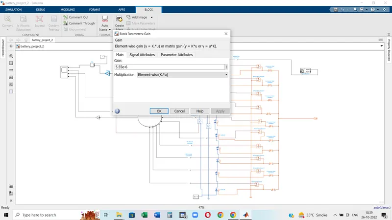
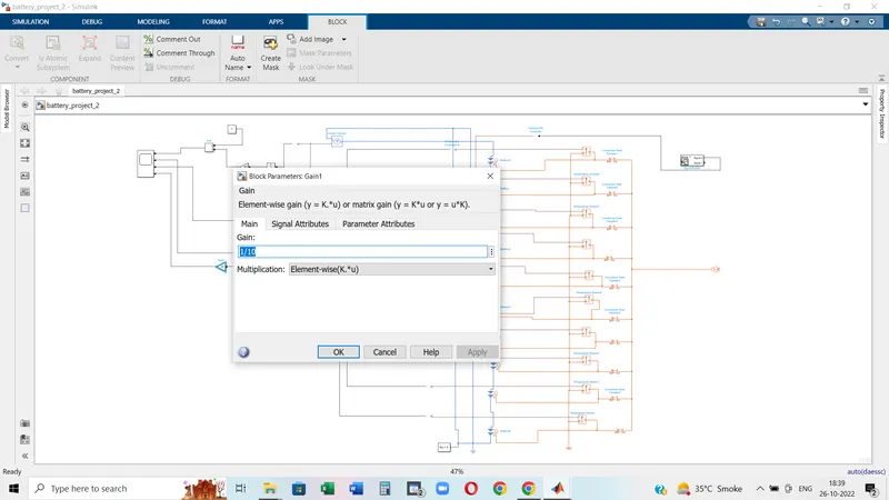
This block has been used two times:

(i) To compute the SOC

(ii) To compute the temperature variations among the batteries connected in series.

The Gain block multiplies the input by a constant value (gain). The input and the gain can each be a scalar, vector, or matrix.
You specify the value of gain in the Gain parameter. The Multiplication parameter lets you specify element-wise or matrix multiplication. For matrix multiplication, this parameter also lets you indicate the order of the multiplicands.
Gain is converted from doubles to the data type specified in the block mask offline using round-to-nearest and saturation. The input and gain are then multiplied, and the result is converted to the output data type using the specified rounding and overflow modes.

9. Add :

This block has been used two times:

(i) To determine the Depth of Discharge

(ii) To add the temperature values of individual battery

The Sum block performs addition or subtraction on its inputs. The Add, Subtract, Sum of Elements, and Sum blocks are identical blocks. This block can add or subtract scalar, vector, or matrix inputs. It can also collapse the elements of a signal and perform a summation.
You specify the operations of the block with the List of signs parameter with plus (+), minus (-), and spacer (|).

10. Constant:

The Constant block generates a real or complex constant value signal. Use this block to provide a constant signal input. The block generates scalar, vector, or matrix output, depending on:

The dimensionality of the Constant value parameter
The setting of the Interpret vector parameters as 1-D parameter

The output of the block has the same dimensions and elements as the Constant value parameter. If you specify for this parameter a vector that you want the block to interpret as a vector, select the Interpret vector parameters as a 1-D check box. Otherwise, if you specify a vector for the Constant value parameter, the block treats that vector as a matrix.

11. Scope:

This block is used to represent the result in a graphical format.

12. Solver Configuration:

Each physical network represented by a connected Simscape™ block diagram requires solver settings information for simulation. The Solver Configuration block specifies the solver parameters that your model needs before you can begin the simulation.
Each topologically distinct Simscape block diagram requires exactly one Solver Configuration block to be connected to it.

13. Thermal Reference:

The Electrical Reference block represents an electrical ground. Electrical conserving ports of all the blocks that are directly connected to ground must be connected to an Electrical Reference block. A model with electrical elements must contain at least one Electrical Reference block.

14. Electrical Reference:

The Thermal Reference block represents a thermal reference point, that is, a point with an absolute zero temperature, with respect to which all the temperatures in the system are determined.

15. Signal Builder:

The Signal Builder block allows you to create interchangeable groups of piecewise linear signal sources and use them in a model. You can quickly switch the signal groups into and out of a model to facilitate testing. In the Signal Builder window, create signals and define the output waveforms. To open the window, double-click the block.

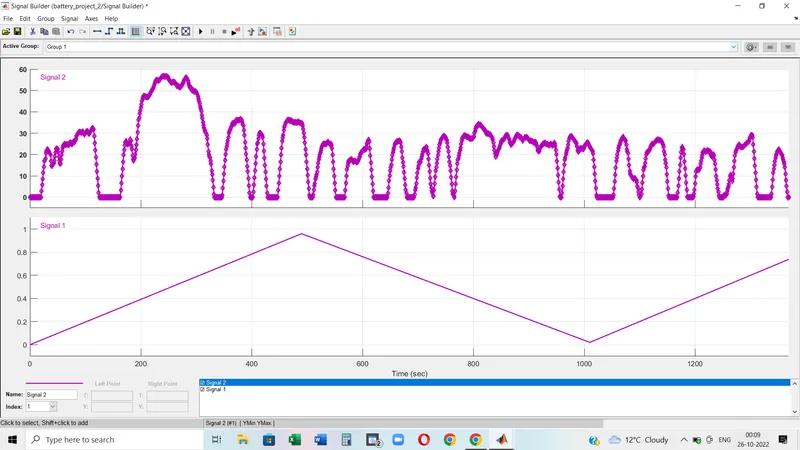
Here for this model two types of signal have been set to determine the SOC level variation for different signals acting on the battery blocks.

Model Execution:

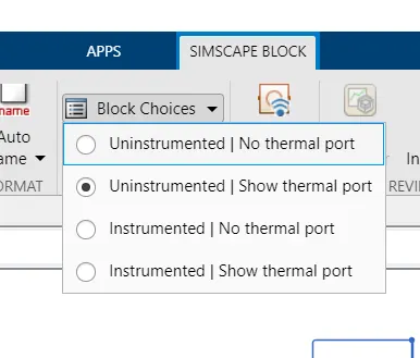
To begin with, we need to generate a battery block and change the necessary parameters as per requirement. In this model diagram, each battery has a thermal port. So to add a thermal port, top of the window of MATLAB, under the 'Simscape Block' section, 'Block choices' is there. Inside that option, Uninstrumented | Show thermal port was selected.

10 number of battery are connected in series. In a series connection, battery pack voltage is added without changing the capacity. To increase the capacity we need to add more strings in parallel.
So here, each battery voltage is fixed at 12 Volt(Nominal Voltage) so the total battery pack voltage is 120 Volt and the capacity is the same as each battery i.e. 50 AH.
After connecting 10 batteries in series, we need to connect the thermal port of the battery.
So from the 'Temperature Source' block, output goes to each battery thermal port through the 'convective heat transfer' block.
A 'Signal Builder' block is used to generate the signal which will decide how the battery will be discharged and the temperature will be risen up.
So via a Controlled Current Source, the signal builder block is connected.
A current sensor is connected in series with the total battery pack.
A voltage sensor is connected in parallel to the battery pack to measure the voltage of the battery pack.
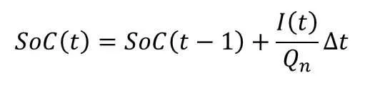
As we have the concern to measure the SOC, here by the Coulomb Counting Method, the SOC is measured, and the output graph is coming on the Scope.
The Coulomb Counting method formula is,
So to determine the Depth of Discharge, the formula will be, 1-(1/C)int(Current)/3600.
The output from the current sensor has been fed to the integration block. Next by gain block (1/50*3600) has been multiplied.

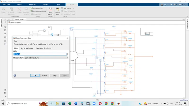
furthermore, by using Add block the output coming from the gain block is subtracted from 1 to determine the Depth of Discharge.
To get the voltage, and current variation the scope block is used.
From a battery, using a temperature sensor, temperature variation is also been measured and put in the scope as the graphical representation.
By changing the temperature at Temperature Source we will get different values of temperature at the battery.
By changing the signal from the signal builder block, we can get different voltage currents and DOD levels.

Result:

In the case of Signal_1

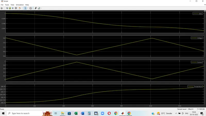
SOC level is left at 0.997 after 1369 seconds.
As per signal 1, during discharge, the maximum current has risen up to 1 Am and then gone to 0.
To maintain the power, when the current is rising up, the magnitude of voltage is coming down simuntenously. As the voltage of each cell was 12 V so the total voltage of the battery pack is 120 V. So in the graph, The voltage started to decrease from 120 V and came to 100 V and then repeated.
The temperature is risen up to 298.18 K after 1369 seconds.

In the case of Signal_2

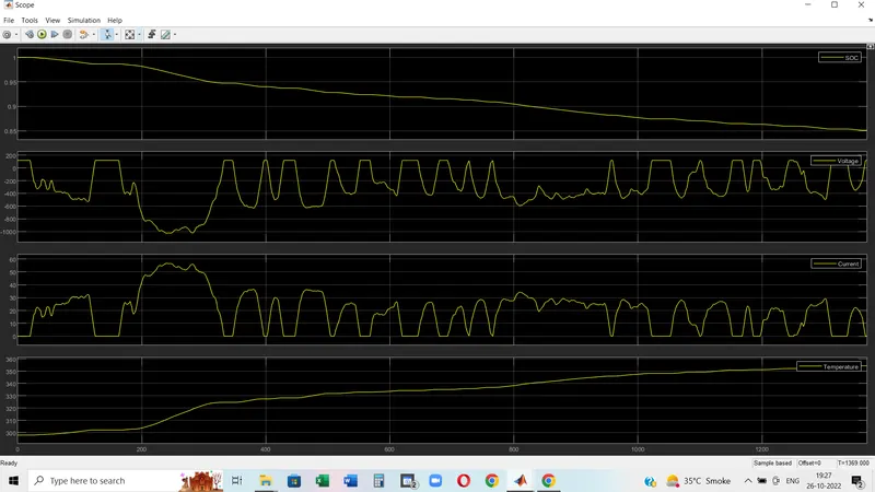
For the same reason here also the voltage started to decrease from 120 V as discussed in the previous case.
Here as per the signal, the current has varied, and to maintain the total power voltage varied in the reverse direction.
Here the temp started to rise from the ambient value 298.15 K and after 1369 seconds it lifted to 345 K. As here input signal is changed so the charge-discharge cycle has also been changed accordingly. For the frequent charge-discharge cycle temp rising is more compared to the previous one.

--------------------------------------------------------------------------------------------------------------------------------------------------------------------------

Project 2 Thermal modeling of battery pack

Ship work like this
in your own course.

Talk to a career counsellor

Ship work like thisin your own course.

Talk to a career counsellor

Ship work like this
in your own course.