Project 2 Thermal modeling of battery pack
For a 10 cell series lithium ion battery model, simulate the thermal effects and compare life cycle performance at various temperatures, charge & discharge rates using MATLAB.
Objective:
- To create a MATLAB model for Lithium ion battery pack of 10 cells connected in series.
- To simulate the thermal effects and compare the performance of charging and discharging at different temperatures.
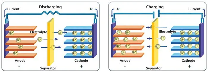
Lithium-ion Battery: Lithium-ion (Li-ion) batteries are an important component of energy storage systems used in various applications such as electric vehicles and portable electronics. Li-ion battery is a type of rechargeable battery composed of cells in which lithium ions move from the negative electrode through an electrolyte to the positive electrode during discharge and back when charging. Li-ion cells use an intercalated lithium compound as the material at the positive electrode and typically graphite at the negative electrode. The cathode can have three different structures that consist of a layered, spinal or olivine structure. Li-ion batteries have a high energy density, no memory effect and low self discharge. Cells can be manufactured to either prioritize energy or power density. There are many chemistries of Li-ion battery, but LFP, NMC, LMO and NCA are four commonly used types. The following figure shows the charging and discharging operation of Li-ion battery.
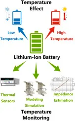
Effect of Cold on Battery: Prolonged exposure to cold temperatures also has a big impact on battery performance and safety. When temperatures drops, the internal resistance of the battery is increased. This means that it requires more effort by the battery to charge, in turn lowering the capacity(Ah). However, it is important to note that the loss of capacity also depends on the charge and discharge rates and effect of the cold weather is different for batteries made with different chemistries. The operating temperatures of batteries are also different based on the type of battery we are working with. For example, LIBs can be charged from 32°F - 113°F and discharged from –4°F - 140°F (however if you operate at such high-temperature levels you do run into the problems mentioned earlier). But Lead-acid batteries can be charged and discharged from -4°F to 122°F. It is very important to be aware of the charging temperatures that a battery can accommodate. If batteries do not operate at the accepted temperature, charge acceptance will be decreased because ion combination will be slower. Forcing high current can build up pressure causing explosions of sealed batteries. The following figure shows the voltage and capacity variations with respect to the different temperatures.
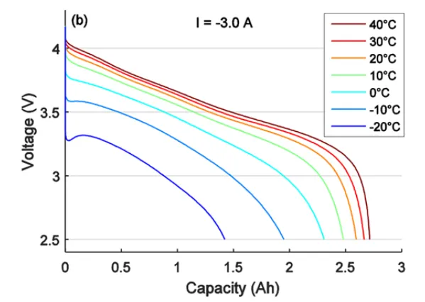
Battery capacity is reduced as temperature goes down, and increased as temperature goes up. This is why your car battery dies on a cold winter morning, even though it worked fine the previous afternoon. If your batteries spend part of the year shivering in the cold, the reduced capacity has to be taken into account when sizing the system batteries. The standard rating for batteries is at room temperature 25°C (about 77° F). At approximately -22° F (-30° C), battery capacity drops to 50%. At freezing, capacity is reduced by 20%. Battery charging voltage also changes with temperature. It will vary from about 2.74V per cell at -40° to 2.3V per cell at 50°C. This is why you should have temperature compensation on charge control if your batteries are outside and/or subject to wide temperature variations.
Internal temperature of the Battery: Thermal mass means that because they have so much mass, they will change internal temperature much slower than the surrounding air temperature. A large insulated battery bank may vary as little as 10°C over 24 hours internally, even though the air temperature varies from 20° to 70°. For this reason, external (add-on) temperature sensors should be attached to one of the +ve plate terminals, and bundled up a little with some type of insulation on the terminal. The sensor will then read very close to the actual internal battery temperature.
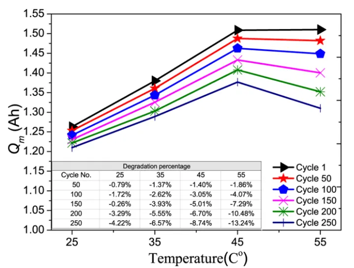
Battery Life at higher temperatures: Even though battery capacity(Ah) at high temperatures is higher, battery life is shortened. Battery capacity is reduced by 50% at -22°F, but battery life increases by about 60%. Battery life is reduced at higher temperatures for every 15°F over 77, battery life is cut in half. The following figure shows the life cycle of the battery according to the variations in C-Rates and with respect to the temperature.
Descripton of Modelling: The following figure shows the MATLAB model of 10 cells connected in series. Where the connection of the cells are divided into two different mocules. Both modules are connected in series. Overall modelling shows the battery pack of 2 modules each module of five cells. Where the signal builder block is taken to give the current signal, which is given to the cotrolled current source block. From there the current signal is given to the both moules. And a temperature source is connected through this we can change the temperature values. And both modules are connected to two different scope blocks which gives the SOC and temperature variations.
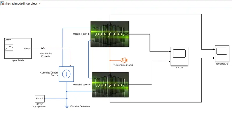
The two modules are constructed in equal manner with equal number of cells in series. For the clear understanding we have taken two modules. The following figure shows the subsystem of modules(1&2).
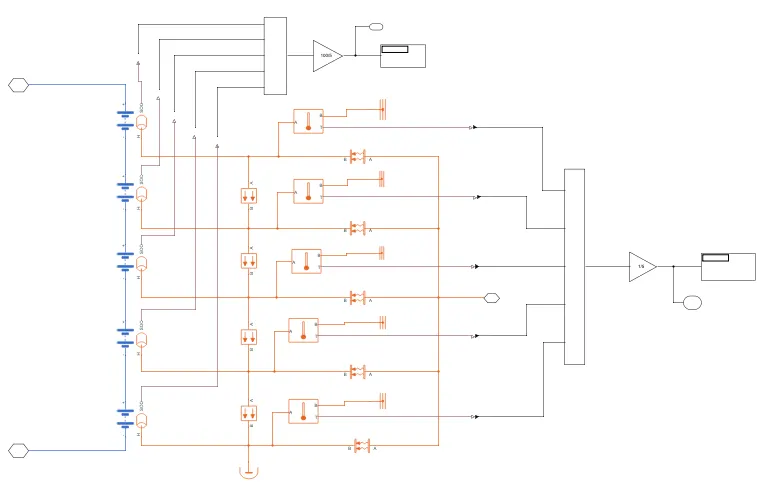
Where the batteries are connected in series manner like the negative terminal of one battery is given to the positive terminal of another battery which is called as series connection. At the battery block we have taken the thermal port and SOC port. The thermal ports are connected with the temperature sensor, Conductive heat transfer and Convective heat transfer block.From the temperature sensor block we can calculate the temperature across the module. Which are given to the addition block and then averaged by gain block, further it gives the value of temperature in display block.
The SOC ports of each battery cell is connected to the add block through the PS-simulink block. Where all the SOC values of cells are get added and then the final SOC will taken from the gain block. Which is also dispayed in the display block after the simulation.
Block used in Modelling: In our model first we have to model the 10 lithium ion cells in a series connection, then will connect the cells to the respective blocks to know the thermal effect of battery pack of 10cells. In the modelling of our project we have used the following blocks.
Battery (Table-based),
Signal builder block,
Controlled current sorce block,
Temperature source block,
Temperature sensor block,
Convective heat transfer block,
Conductive heat transfer block,
Thermal reference,
Electrical reference,
Perfect insulator,
Simulink-PS converter,
PS-Simulink converter,
Gain block,
Add block,
Scope block,
Display block,
Solver configuration block.
Will see the representation of each block in our model.
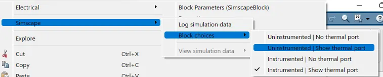
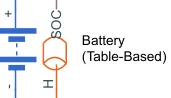
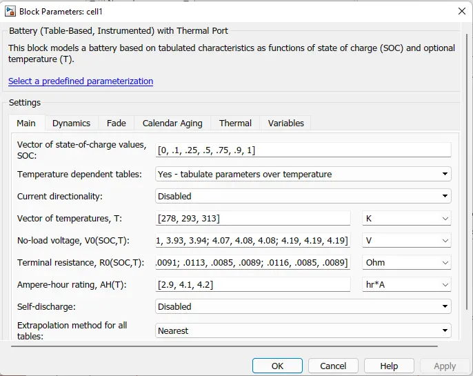
Battery (table based): Battery (table based) models a battery based on tabulated characteristics as functions of SOC and temeperature. Here we have taken all the default parameters. But to select the thermal port, right click on the block and goto simscape option then block choices and later select the second option(Uninstrumented show thermal port). Repeat the same procedure again and this time select the 4th option(Instrumented show thermal port). Then the SOC and thermal port will appears. Which is shown in the following figures.
The following figure shows the parameters of the Battery block. Which is common for all battery blocks.
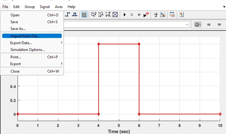
Signal builder block: Signal builder block is used to create the signals as per our data or we can import the files to it rather than making all the points(if it consists more values). Here we are taking the UDDS data to build the signal. For this i have imported a file through the import option which is shown in the following figure.
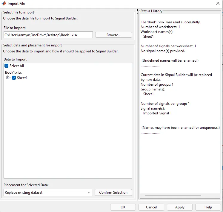
By clicking on the import from file option, the following window will appears. Where by clicking on the browse option, we can select the excel file which represents the UDDS data. After that at placement for selected data select the option as replace existing datsheet then click on ok button.
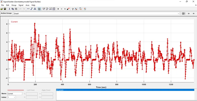
After clicking on Ok button, the following plot will appears which is a UDDS current data plot. Which is used in our model to observe the variations in charge and discharge rates.
Controlled current source: The controlled current source block represents an ideal current sorce that is powerful enough to maintain the specified current through it regardless of the voltage across the source. Where the controlled current source block is connected across the battery pack (10cells). The following figure shows the controlled current source block.

To its physical port we are giving the current signal from the signal builder block.
Temperature source block: The Temperature source block represents an ideal source of thermal energy that is powerful enough to maintain specified temperature at its outlet regardless of the heat flow consumed by the system. The source generates constant absolute temperature, defined by the temperature parameter value. Through this block will can give the different temperatures to the battery pack. It is connected as common for both Modules 1&2.

Temperature sensor block: The Temperature sensor block represents an ideal temperature sensor, i.e, a device that determines the temperature differential measured between two points without drawing any heat. Connections A and B are thermal conserving ports that connect to the two points where temperature is being monitored. Port T is a physical signal port that outputs the temperature differential value.

Temperature sensor block is connected across each cell, to measure the temperature of each cdll. And that temperatures are given to the add block then it is averaged to give final temperature.
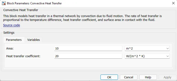
Convective heat transfer block: The Convective heat transfer block represents a heat transfer by convection between 2 bodies by means of fluid motion. The transfer is governed by the Newton law of cooling and is described with the equation given below,
Q = k×A×(TA - TB)
where,
Q = Heat flow,
k = Convection heat transfer coefficient
A = Surface area
TA and TB are temperatures of the bodies.
The following image shows the Convective heat transfer block.

The following figure shows the parameters modeled in Convective heat transfer block.
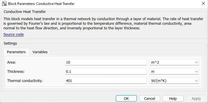
Conductive heat transfer block: The Conductive heat transfer block represents a heat transfer by conduction between 2 layers of the same material. The transfer is governed by the Fourier law and is described with the equation given below,
Q=k·AD(TA−TB)
where,
Q = Heat flow,
k = Material thermal conductivity,
A = Area normal to the heat flow direction,
D = Distance between layers
TA, TB are temperatures of the layers.
The following image shows the onductive heat transfer block.

The following figure shows the parameters modeled in Conductive heat transfer block.
Thermal reference: The Thermal reference block represents a thermal reference point, i.e, a point with an absolute zero temperature, with respect to which all the temperatures in the system are determined. The following image shows the Thermal reference block.

Electrical reference: The electrical reference block represnts an electrical ground. This block has only one electrical conserving port. Electrical conserving ports of all theelectrical block that are directly connected to ground must be connected to an electrical reference block. Following images shows the figure of electrical reference block.

Perfect insulator: The Perfect insulator block represents a thermal element with perfect insulation and no thermal mass. We can use this block as an insulation for thermal ports to prevent heat exchange with the environment and to model an adiabatic process. The following image shows the Perfect insulator block. Which is connected common to all the thermal blocks in our model.

PS-Simulink converter: The PS-simulink block converts a physical signal into a simulink output signal. We used this block to connect the outputs of a physical network blocks to simulink blocks. The following images shows the PS-simulink converter.

Simulink-PS converter: The Simulink-PS block converts a simulink signal into a physical output signal. We used this block to connect the outputs of a simulink network blocks to physical blocks. The following images shows the Simulink-PS converter when it is unconnected.

When it is connected to other blocks, the Simulink-PS converter looks like in the following image.

Gain: The gain block multiplies tha input by a constant value. The following image shows the gain block. It has only one input and output port. In our project we have used gain blocks across the SOC measurement and Temperature measurement. At SOC measurement it is taken as 100/5 for module 1&2. At temperature measurment it is taken as 1/5 to calculate the average temperature.

Add Block: The addition block is used to add the input values and give the result through its single output. Here all the temperature measurement ports and all the SOC measurement ports are given to two different add blocks. Then giving its output to the gain block which further gives the result of SOC and Temperature.
Scope: The following image shows the scope block. Through the scope block we can observe the resultant plots. We can add the additional ports to view the number of plots in one scope block. We can select the legend option in the plot to view the name of the plot. Ans we can set the layout to view the different plots.

Display block: The Display block shows the value of the input dats. We can specify the frequency of the display. For numeric input data, we can also specify the format of display. The following figure shows the display block. In our model it is connected to view the SOC and Temperature.
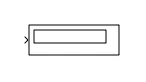
Solver configuration: The solver configuration block is shown in the following image. Each physical network represented by a connected simscape block diagram requires solver settings information for simulation. It specifies the solver parameters that our model needs before we can begin simulation. Each topologically distinct simscape block diagram requires exactly one solver configuration black to be connected to it.

The block has one conserving port. We can add this block anywhere on a physical network circuit by creating a branching point and connecting it to the only port of the solver configuration block. In our model i have connected the solver configuration block at the common ground terminal.
Simulation & Results: Now we are going to simulate the model we have created with two modules of 10 cells series connection. So before the simulation we have to give the some temperature to the battery pack through the temperature sensor block.
First we are giving the temperature as 300K, then simulated for 1369seconds as per our current signal. Then the module gets simulated and shows the following results in the display blocks.
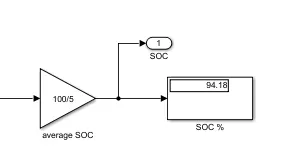
In the above figure it is showing the percentage of SOC of module (1&2). Bothe modules will gives the same result because we have connected them in a similar way. So the value of %SOC at 300K temperature is 94.18%. The temperature value is also we can observe through the respective display block which is shown in the following figure.
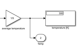
The resultant plots can be observed through the Scope blocks. Where both modules are giving the equal results because of their similar connection and similar parameters. That is why the two plots are plotted at same variation. The Yellow plot gives the result of Module 1 and the Blue plot gives the result of Module 2.
The following figure shows the %SOC plot of both modules at 300K temperature.
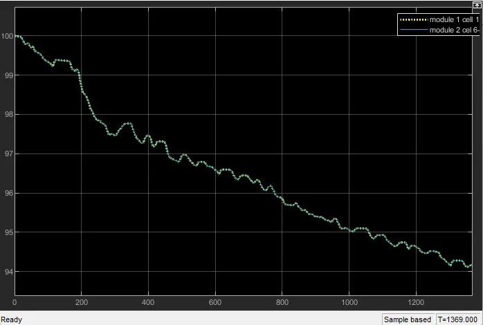
In the above we can observe that, as per our current signal there is charging and discharging conditions happen. That is when current is increasing then there will be a discharging condition in SOC as vehicle is using its capcity. And when the current value is decrease that is the condition where the battery gets charged up. After the completion of given current signal at 1369seconds the %SOC reaches to around 94%. Which is already displayed in the SOC display block.
The following plot shows the temperature variation of the battery pack of two modules.
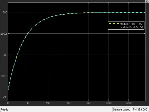
In the above plot we can observe that, before simulating the model, the temperature of the battery pack is around 298K. After the simulation, the temperature rises gradually and reaches to 300K at around 300seconds. Then maintained its constant temperature as it is the maximum temperature we have given through the temperature source.
Now we are giving the temperature as 400K, then simulated for 1369seconds as per our current signal. Then the module gets simulated and shows the following results in the display blocks.
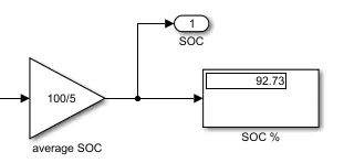
In the above figure it is showing the percentage of SOC of module (1&2). Both modules will gives the same result as already mentioned. So the value of %SOC at 400K temperature is 92.73%. The temperature value is also we can observe through the respective display block which is shown in the following figure.
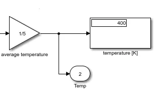
The resultant plots can be observed through the Scope blocks. The following figure shows the %SOC plot of both modules at 400K temperature.
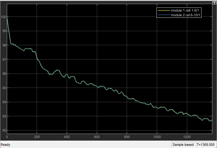
In the above we can observe that, as per our current signal there is charging and discharging conditions happen as happened in the previous case. After the completion of given current signal that is at 1369seconds the %SOC reaches to around 92.7%. Which is already displayed in the SOC display block.
The following plot shows the temperature variation of the battery pack of two modules.
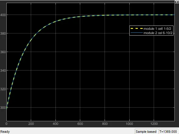
In the above plot we can observe that, before simulating the model, the temperature of the battery pack is around 300K. In the before simulation we have taken 300K so that is why the plot starting from 300K temperature. After the simulation, the temperature rises gradually and reaches to 400K at around 300seconds. Then maintained its constant temperature as it is the maximum temperature we have given through the temperature source.
Conclusion: MATLAB model for Lithium ion battery pack of 10cells (connected in series) has been created. The thermal effects on the battery pack has been simulated. From the observation of model we have created it can be say that, when the temperature value increases then its respective charging and discharging capacity decreases due to the heat generated in the batteries. To observe this change we have simulated the model for two different temperatures, so it can be observed that there is a decrease in the %SOC when the temperature value increased. For the efficient operation of the battery pack, proper thermal management is required.
- V Gopi Krishnagood morning, madam. Can you please update the Signal builder block Excell sheet Link for reference purpose madam. Thank and regards. V Gopi Krishna