Project 2 - Rankine cycle Simulator
OBJECTIVE:
- Create a Rankine Cycle Simulator using OCTAVE/MATLAB.
- The code should calculate the state points of the Rankine Cycle (any type of your choice) based on user inputs.
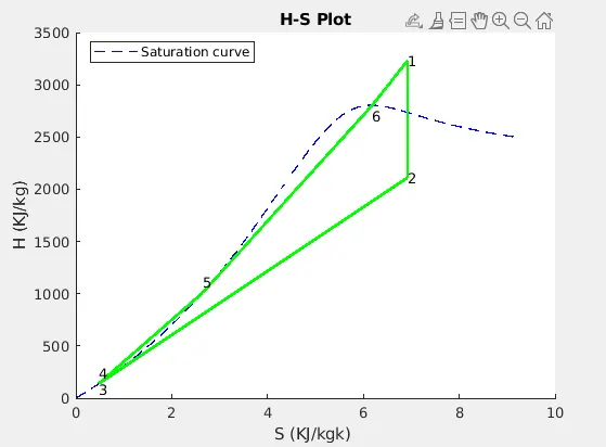
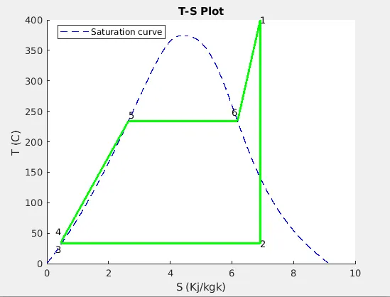
- Plot the corresponding T-s and h-s plots for the given set of inputs. Title and axes labels are a must, while legends could be used if necessary.
THEORY:
Rankine Cycle:
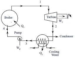
Rankine Cycle is one of the standard steam power plant cycles. It consists of an isentropic expansion process taking place in turbine and an isentropic compression process that occurs in the compressor, alternating two isobaric processes - heat addition in boiler and heat rejection in condenser. The following diagram shows a rankine cycle:
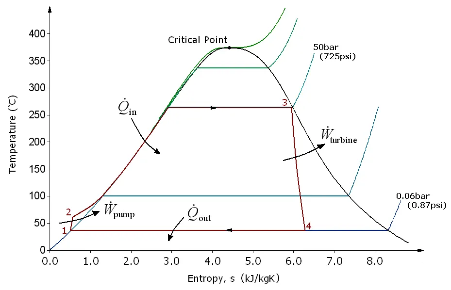
An example rankine cycle on T-S plot:
CODE:
In our program we will take user input for three parameters - Pressure at Turbine inlet, Temperature at Turbine inlet and Pressure at Condenser outlet respectively:
%% Taking User Input:
p1 = input('\nEnter the Pressure at Turbine Inlet, p1(bar) = ');
T1 = input('\nEnter the Temperature at Turbine Inlet, T1(degree.C) = ');
p2 = input('\nEnter the Temperature at Condenser Inlet, p2(bar) = ');
Based on these parameters we will optain the required state properties from the XSteam file which acts as a steam table:
%% Obtaining necessary properties from Xsteam:

h1 = XSteam('h_pT', p1, T1);        % Enthalpy f(P,T)
s1 = XSteam('s_pT', p1, T1);        % Entropy  f(P,T)
sf2 = XSteam('sL_p', p2);           % Saturated liquid Entropy
sg2 = XSteam('sV_p', p2);           % Saturated Vapour Entropy
hf2 = XSteam('hL_p', p2);           % Saturated Liquid Ethalpy
hg2 = XSteam('hV_p', p2);           % Saturated Vapour Enthalpy
vf2 = XSteam('vL_p', p2);           % Saturated Liquid Volume
Obtaining Data from XSteam:
To obatin values from XSteam, following syntax should be followed:
property_variable = XSteam('a_b', c);where, a = name of the property (h, s, T etc.) followed by the phase of water (v = vapour, L = gas).
b = the property a is dependent on (p,T etc.)
c = the value of b at which we want to find out b
the nomenclature for a_b can be taken from the XSteam header and used accordingly. Example for Enthalpy:
%Enthalpy
%hV_p	Saturated vapour enthalpy
%hL_p	Saturated liquid enthalpy
%hV_T	Saturated vapour enthalpy
%hL_T	Saturated liquid enthalpy
%h_pT	Entalpy as a function of pressure and temperature.
%h_ps	Entalpy as a function of pressure and entropy.
%h_px	Entalpy as a function of pressure and vapour fraction
%h_prho	Entalpy as a function of pressure and density. Observe for low temperatures (liquid) this equation has 2 solutions.
%h_Tx	Entalpy as a function of temperature and vapour fraction
Computing required parameters:
Next, we will use the parameters we obtained from XSteam to calculate other parameters and cycle performance parameters as well using thermodynamic relations:
%% Computing Required Properties:
x2 = (s1-sf2)/(sg2-sf2);            % Dryness Fraction
h2 = hf2 + (x2*(hg2-hf2));          % Enthalpy at Turbine outlet

Wp = vf2*(p1-p2);                   % Work Done (Pump)
Wt = h1 - h2;                       % Work Done (turbine)
Wnet = Wt - Wp;                     % Net Work Done

h4 = Wp + hf2;                      % Enthalpy at Pump Outlet

Qin = h1 - h4;                      % Heat Consumed
Qout = h2 - hf2;                    % Heat Rejected

eff_T = Wnet/Qin;                   % Thermal Efficiency
SSC = (3600/Wnet);                  % Specific Heat COnsumption (kJ/kWh)
BWR = Wt/Wp;                        % Back Work Ratio
Finally, we will calculate the properties at all the state points to plot easily:
%% Computing properties at other state points for plotting:
% Entropy
s2 = s1;
s3 = sf2;
s4 = s3;
s5 = XSteam('sL_p', p1);
s6 = XSteam('sV_p', p1);

% Enthalpy
h3 = hf2;
h4 = h3;
h5 = XSteam('hL_p', p1);
h6 = XSteam('hV_p', p1);

% Temperature:
Cp = XSteam('Cp_ps',p1,s4);        % Specific Heat Capacity at Constant Pressure
Cv = XSteam('Cv_ps',p1,s4);        % Specific Heat Capacity at Constant Volume
k = Cp/Cv;                         % Adiabatic Constant

T2 = XSteam('Tsat_p', p2);
T3 = T2;
T4 = T3*((p1/p2)^((k-1)/k));
T5 = XSteam('Tsat_p', p1);
T6 = T5;

% Saturation Curve:
T = linspace(1,375,1000);

for i = 1:length(T)
    sf(i) = XSteam('sL_T', T(i));
    sg(i) = XSteam('sV_T', T(i));
    hf(i) = XSteam('hL_T', T(i));
    hg(i) = XSteam('hV_T', T(i));
end
After obtaining all the values we will plot the H-S and T-S charts and display the major results in the terminal.
Complete Program:
% Rankine Cycle Simulator

close all     % Close Open Plots
clear all     % Clear Workspace
clc           % Clear Command Window


%% Display Cycle Process to help with User input:
fprintf('RANKINE CYCLE\n');
fprintf('1-2 is Isentropic Expansion in the turbine\n');
fprintf('2-3 is constant pressure heat removal in the condenser\n');
fprintf('3-4 is Isentropic compression in the pump\n');
fprintf('4-1 is Constant pressure heat addition in the boiler\n');

%% Taking User Input:
p1 = input('\nEnter the Pressure at Turbine Inlet, p1(bar) = ');
T1 = input('\nEnter the Temperature at Turbine Inlet, T1(degree.C) = ');
p2 = input('\nEnter the Temperature at Condenser Inlet, p2(bar) = ');

%% Obtaining necessary properties from Xsteam:

h1 = XSteam('h_pT', p1, T1);        % Enthalpy f(P,T)
s1 = XSteam('s_pT', p1, T1);        % Entropy  f(P,T)
sf2 = XSteam('sL_p', p2);           % Saturated liquid Entropy
sg2 = XSteam('sV_p', p2);           % Saturated Vapour Entropy
hf2 = XSteam('hL_p', p2);           % Saturated Liquid Ethalpy
hg2 = XSteam('hV_p', p2);           % Saturated Vapour Enthalpy
vf2 = XSteam('vL_p', p2);           % Saturated Liquid Volume

%% Computing Required Properties:
x2 = (s1-sf2)/(sg2-sf2);            % Dryness Fraction
h2 = hf2 + (x2*(hg2-hf2));          % Enthalpy at Turbine outlet

Wp = vf2*(p1-p2);                   % Work Done (Pump)
Wt = h1 - h2;                       % Work Done (turbine)
Wnet = Wt - Wp;                     % Net Work Done

h4 = Wp + hf2;                      % Enthalpy at Pump Outlet

Qin = h1 - h4;                      % Heat Consumed
Qout = h2 - hf2;                    % Heat Rejected

eff_T = Wnet/Qin;                   % Thermal Efficiency
SSC = (3600/Wnet);                  % Specific Heat COnsumption (kJ/kWh)
BWR = Wp/Wt;                        % Back Work Ratio

%% Computing properties at other state points for plotting:
% Entropy
s2 = s1;
s3 = sf2;
s4 = s3;
s5 = XSteam('sL_p', p1);
s6 = XSteam('sV_p', p1);

% Enthalpy
h3 = hf2;
h4 = h3;
h5 = XSteam('hL_p', p1);
h6 = XSteam('hV_p', p1);

% Temperature:
Cp = XSteam('Cp_ps',p1,s4);        % Specific Heat Capacity at Constant Pressure
Cv = XSteam('Cv_ps',p1,s4);        % Specific Heat Capacity at Constant Volume
k = Cp/Cv;                         % Adiabatic Constant

T2 = XSteam('Tsat_p', p2);
T3 = T2;
T4 = T3*((p1/p2)^((k-1)/k));
T5 = XSteam('Tsat_p', p1);
T6 = T5;

% Saturation Curve:
T = linspace(1,375,1000);

for i = 1:length(T)
    sf(i) = XSteam('sL_T', T(i));
    sg(i) = XSteam('sV_T', T(i));
    hf(i) = XSteam('hL_T', T(i));
    hg(i) = XSteam('hV_T', T(i));
end

%% PLOTS:
% T-S Diagram:
figure(1)
hold on
plot(sf, T, 'b--','linewidth',1)
plot(sg, T, 'b--','linewidth',1)

plot([s1 s2], [T1 T2], 'g', 'linewidth', 2)
plot([s2 s3], [T2 T3] ,'g', 'linewidth', 2)
plot([s3 s4], [T3 T4], 'g', 'linewidth', 2)
plot([s4 s5], [T4 T5], 'g', 'linewidth', 2)
plot([s5 s6], [T5 T6], 'g', 'linewidth', 2)
plot([s6 s1], [T6 T1], 'g', 'linewidth', 2)

% State Points
text(s1, T1, '1')
text(s2, T2, '2')
text(s3-0.2, T3-10, '3')
text(s4-0.2, T4+15, '4')
text(s5, T5+10, '5')
text(s6-0.2, T6+15, '6')

title('T-S Plot')
xlabel('S (Kj/kgk')
ylabel('T (C) ')
legend('Saturation curve')


% H-S Diagram
figure(2)
hold on
plot(sf, hf, 'b--', 'linewidth', 1)
plot(sg, hg, 'b--',  'linewidth', 1)
plot([s1 s2], [h1 h2], 'g', 'linewidth', 2)
plot([s2 s3], [h2 h3], 'g', 'linewidth', 2)
plot([s3 s4], [h3 h4], 'g', 'linewidth', 2)
plot([s4 s5], [h4 h5], 'g', 'linewidth', 2)
plot([s5 s6], [h5 h6], 'g', 'linewidth', 2)
plot([s6 s1], [h6 h1], 'g', 'linewidth', 2)

% State Points:
text(s1, h1, '1')
text(s2, h2, '2')
text(s3, h3-50, '3')
text(s4, h4+100, '4')
text(s5, h5+100, '5')
text(s6, h6-100, '6')

title('H-S Plot')
xlabel('S (KJ/kgk) ')
ylabel('H (KJ/kg)')
legend('Saturation curve')

%% Display Results in Terminal
disp(' RESULTS');
fprintf('At State Point 1:\n');
fprintf('p1 = %f bar\n', p1);
fprintf('T1 = %f C\n', T1);
fprintf('h1 = %f KJ/kg\n', h1);
fprintf('s1 = %f KJ/kgK\n\n', s1);
fprintf('At State Point 2:\n');
fprintf('p2 = %f bar\n', p2);
fprintf('T2 = %f C\n', T2);
fprintf('h2 = %f kJ/kg\n', h2);
fprintf('s2 = %f kJ/kgK\n', s2);
fprintf('x2 = %f\n\n', x2);
fprintf('At State Point 3:\n');
fprintf('p3 = %f bar\n', p2);
fprintf('T3 = %f K\n', T3);
fprintf('h3 = %f kJ/kg\n', h3);
fprintf('s3 = %f kJ/kgK\n\n', s3);
fprintf('At State Point 4:\n');
fprintf('p4 = %f bar\n', p1);
fprintf('T4 = %f K\n', T4);
fprintf('h4 = %f KJ/kg\n', h4);
fprintf('s4 = %f kJ/kgK\n\n', s4);
fprintf('Turbine Work = %f kJ/kg\n', Wt);
fprintf('Pump Work = %f kJ/kg\n', Wp);
fprintf('Wnet = %f kJ/kg\n', Wnet);
fprintf('Thermal Efficiency = %f %%\n', eff_T);
fprintf('S.S.C = %f kJ/kWh\n', SSC);
fprintf('Back Work Ratio = %f', BWR);
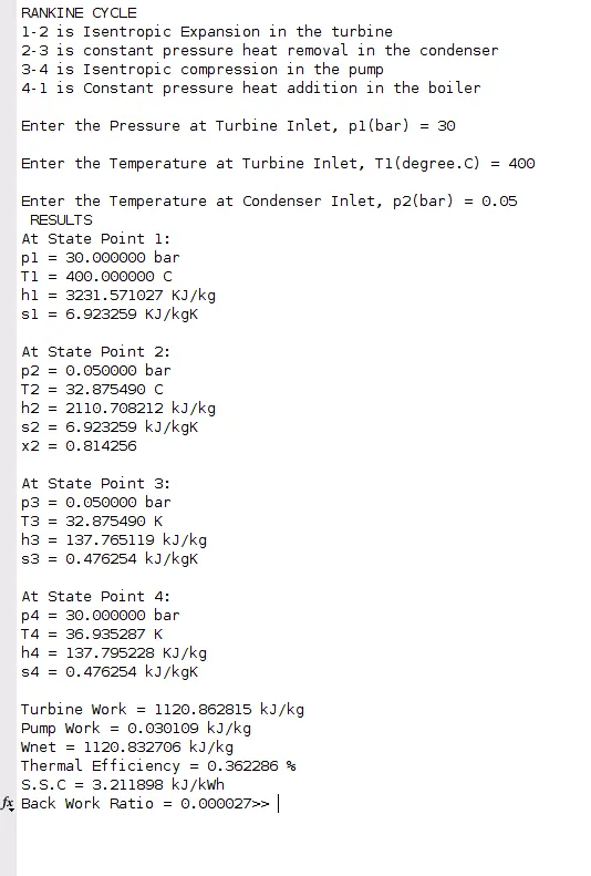
RESULTS:
T-S Plot:
H-S Plot: