Project 2 - Rankine cycle Simulator

Rankine Cycle

Rankin Cycle is an ideal mechanical cycle that convert heat energy to mechanical energy. The system mainly consists of boiler, turbine, condenser, and a pump. The process consists of two adiabatic process and two isobaric process. The Rankine cycle is used to compare by rating the thermodynamic process standards in a steam power plant.

Main Code

clear all
close all
clc

%Rankin Cycle


%Input
T1 = input('Enter Steam Inlet Temperature [in degree Celcius]:- ') ; %degree Celcius
clc
P1 =  input('Enter Input Pressure of steam Entering the Turbine[in bar]:- ') ; %bar
clc
P2 = input('Enter the Pressure of Outlet Steam Pressure from Turbine[in bar]:- '); %bar
clc

%State-1
h1 = XSteam('h_pT',P1,T1);
s1 = XSteam('S_pT',P1,T1);
T_sat1 = XSteam('Tsat_p', P1);
h_f1 = XSteam('hL_p',P1);
h_g1 = XSteam('hV_p',P1);
s_g1 = XSteam('sV_p', P1);
s_f1 = XSteam('sL_p', P1); 


%State-2
h_f2 = XSteam('hL_p',P2);
h_g2 =  XSteam('hV_p',P2);
s_g2 = XSteam('sV_p', P2);
s_f2 = XSteam('sL_p', P2);
h_fg2 = h_g2-h_f2;   s_fg = s_g2-s_f2;
T_sat2 = XSteam('Tsat_p', P2);
s2 = s1;
%Expression to calculate the dynens fraction
x = (s2-s_f2)/s_fg;

%Entalpy at state-2
h2 = h_f2+x*h_fg2;

T2 = XSteam('T_ph',P2,h2);

%State - 3
T3 = T2;
P3 = P2 ;
h3 = h_f2;
s3 = s_f2;

%state - 4
P4 = P1;
s4 = s3;
h4 = XSteam('h_ps',P4,s4);
T4 = XSteam('T_ph',P4,h4);
h_f4 = XSteam('hL_p',P4);
h_g4 = XSteam('hV_p',P4);

%4s
T_4s = XSteam('T_ps',P1,s3);

%Calculations
%Heat Added
q_in = h1 -h4;

%Work done
w_t = h1-h2;   %Turbaine
w_p = h4-h3;    %Pumb
w_net = w_t-w_p;  %Net

%Work Ratio
w_r = (w_net)/w_t; 

%Back Work Ratio
w_b = w_p/w_t;

%efficency
e_th = (w_net/q_in)*100;

%Specific Stream Consumption(Stream Rate)
ssc = 1/w_net;

%Heat Rate
h_r = 1/e_th;  %q_in/w_net

%\\\\\\\\\\\\\\\\\\\Plot Graph

t = linspace(0,500,500);

%\\\\\\\\\\\\\\\\\\\\\\Plot T-s Diagram
figure(1)

for i = 1:length(t)
sL(i) = XSteam('sL_T',t(i));
sV(i) = XSteam('sV_T',t(i));
end

%Saturation curve
hold on;
plot(sL,t,'linewidth',2.5,'color',[0 0 1]);  %Saliration Liqued Line
plot(sV,t,'linewidth',2.5,'color',[0 0 1]);  %Saturation Vapour Line

%Process Isentropic expansion
plot([s1,s2],[T1 T2],'linewidth',2,'color',[0 1 0]);
%plot(s3,T_4s,'marker','*');
%plot([s2 s3], [T2 T3],'linewidth',2,'color', [0 0 0]);

%constant Pressure line at P1
for k=1:length(t)
s_satP1(k)=XSteam('s_pT',P1,t(k));
end
plot(s_satP1,t,'linewidth',0.5,'color',[0 0 0]);  %P1

%Constant Pressure curve at P2
for k=1:length(t)
   s_satP2(k) = XSteam('s_pT',P2,t(k)); 
end
plot(s_satP2,t,'linewidth',0.5,'color',[0 0 0]);   %P2



T0 = linspace(T1, T_4s, 500);
for j = 1:length(T0)
 S_satP1(j) = XSteam('s_pT',P1,T0(j)); 
end
plot(S_satP1,T0,'linewidth',2,'color',[0 1 0]); %Process 4s-1

if x>1
T3 = T_sat2;
plot([s2 s_g2 s3 s4],[T2,T_sat2 T3 T_4s],'linewidth',2,'color',[0 1 0]) %Process 2-3

else
plot([s2 s3 s4],[T2 T3 T_4s],'linewidth',2,'color',[0 1 0]);  %Process 2-3
end
 
plot([s3 s3], [T3 T_4s],'linewidth',2,'color',[0 1 0]);  %Process 3-4s
%plot([s_f1, s_g1], [T_sat1 T_sat1], 'linewidth',2,'color',[0 1 0]);
xlabel('Entropy[KJ/mol-C]')
ylabel('Temprature[C]')
title('T-s Diagram');
grid on;

%\\\\\\\\\\\\\\\\\\\h-s Diagram
figure(2);
hold on;

%Saturation curve
for i=1:length(t)
plot(XSteam('sL_T',t(i)),XSteam('hL_T',t(i)),'.','color','b')
plot(XSteam('sV_T',t(i)),XSteam('hV_T',t(i)),'.','color','b')
end

%h-s Curve
plot([s1 s2 s3 s4 s1],[h1 h2 h3 h4 h1],'linewidth',2,'color','g')
xlabel('Entropy[kJ/mol-C]'); ylabel('Enthalpy[kJ]')
grid on;
title('h vs s Diagram');

%Display
fprintf('State Vatiables\n');
fprintf('State -1[Turbain Inlet]\n');
fprintf('----------------------------\n');
fprintf('Pressure P1 = %f bar\n',P1);
fprintf('Temperature T1 = %f ^0C\n',T1);
fprintf('Enthalpy h1 = %f kJ\n', h1);
fprintf('Entropy s1 = %f kJ/mol-0C\n', s1);
fprintf('******************************\n');

fprintf('State - 2 [Turbain Outlet]\n');
fprintf('----------------------------\n');
fprintf('Pressure P2 = %f bar\n',P2);
fprintf('Temperature T2 = %f C\n',T2);
fprintf('Enthalpy h2 = %f kJ\n', h2);
fprintf('Entropy s2 = %f  kJ/mol-C\n', s2);
fprintf('******************************\n');

fprintf('State - 3 [Condenser Outlet]\n');
fprintf('----------------------------\n');
fprintf('Pressure P3 = %f bar\n',P3);
fprintf('Temperature T3 = %f C\n',T3);
fprintf('Enthalpy h3 = %f kJ\n', h3);
fprintf('Entropy s3 = %f kJ/mol_C\n', s3);
fprintf('******************************\n');

fprintf('State - 4 [Pump Outlet/ Boiler Inlet]\n');
fprintf('----------------------------\n');
fprintf('Pressure P4 = %f bar\n',P4);
fprintf('Temperature T4 = %f C\n',T4);
fprintf('Enthalpy h4 = %f kJ\n', h4);
fprintf('Entropy s4 = %f kJ/C-mol\n', s4);
fprintf('******************************\n');

%Display_Cycle Mechanical Properties
fprintf('Mechanical Propertices\n');
fprintf('----------------------------\n');
fprintf('Amount of Heat Added to the system: %f kJ\n', q_in);
fprintf('Turbin Work: %f kJ\n', w_t);
fprintf('Pump Work: %f kJ\n', w_p);
fprintf('Thermal Efficiency: %f %\n', e_th);
fprintf('Net Work Done: %f kJ\n', w_net);
fprintf('Stream Rate: %f kg/C_Ws\n', ssc);
fprintf('Work Ratio: %f\n', w_r);
fprintf('Back Work Ratio: %f\n', w_b);
fprintf('Heat Rate: %f kJ/C_Ws\n',h_r);
fprintf('******************************\n');

Result

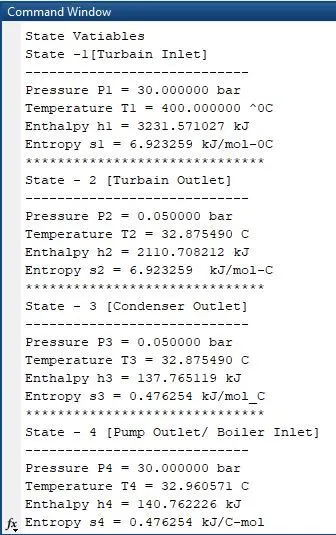
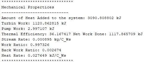
Graph

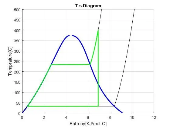
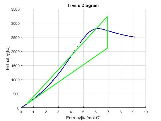
Explanation

Starting with clearing the screen, closing all the plots, and erasing all the inputs or variables saved.

clear all

close all

clc

%Rankin Cycle

Some state variable of the turbine is saved on a variable. The variables, are stored using a ‘input’ command from the commander. On using the ‘input’ command the variable scalar quantity can be change on each time when the code runs. The ‘clc’ command is used in between the variable to clear the screan after entering a variable.

%Input

T1 = input('Enter Steam Inlet Temperature [in degree Celcius]:- ') ; %degree Celcius

clc

P1 =  input('Enter Input Pressure of steam Entering the Turbine[in bar]:- ') ; %bar

clc

P2 = input('Enter the Pressure of Outlet Steam Pressure from Turbine[in bar]:- '); %bar

clc

State – 1 variables are founded using given inputs. The ‘XSteam’ is a predefined function that is used to call the temperature, entropy, and enthalpy values of a state using some proper references which are pre-defined variables. (state -1 heat addition to the turbine from boiler)

%State-1

h1 = XSteam('h_pT',P1,T1);

s1 = XSteam('S_pT',P1,T1);

T_sat1 = XSteam('Tsat_p', P1);

h_f1 = XSteam('hL_p',P1);

h_g1 = XSteam('hV_p',P1);

s_g1 = XSteam('sV_p', P1);

s_f1 = XSteam('sL_p', P1);

Using the state – 1 variables and the given inputs state – 2 variables are determined. The ‘XSteam’ function is called out to determine the saturation variable here.

%State-2

h_f2 = XSteam('hL_p',P2);

h_g2 =  XSteam('hV_p',P2);

s_g2 = XSteam('sV_p', P2);

s_f2 = XSteam('sL_p', P2);

h_fg2 = h_g2-h_f2;   s_fg = s_g2-s_f2;

T_sat2 = XSteam('Tsat_p', P2);

s2 = s1;

The dryness fraction is calculated using the entropy variables.

%Expression to calculate the dryness fraction

x = (s2-s_f2)/s_fg;

The enthalpy is calculated using the expression ‘H = H_g – x*(H_fg)’ it can also be calculated by the expression ‘H=H_f + x(H_fg)’. (Here H is the enthalpy at a state, h_f is the enthalpy of saturated liquid, h_g is the enthalpy of saturated vapor, and h_fg is the difference between the enthalpy of saturation.)

%Entalpy at state-2

h2 = h_f2+x*h_fg2;

The temperature at state – 2 is calculated by calling the ‘XSteam’ function with references as pressure and enthalpy at state -2.

T2 = XSteam('T_ph',P2,h2);

State – 3 variables are calculated.

%State - 3

T3 = T2;

P3 = P2;

h3 = h_f2;

s3 = s_f2;

State – 4 variables are calculated.

%state - 4

P4 = P1;

s4 = s3;

h4 = XSteam('h_ps',P4,s4);

T4 = XSteam('T_ph',P4,h4);

h_f4 = XSteam('hL_p',P4);

h_g4 = XSteam('hV_p',P4);

The ‘XSteam’ function is called out to calculate the temperature at outlet of the pump.

%4s

T_4s = XSteam('T_ps',P1,s3);

%Calculations

Heat added to the system (Boiler) is calculated using the expression Q = H₄-H₁.

%Heat Added

q_in = h1 -h4;

Work Done by the turbine, pump, and net work-done is calculated.

%Work done

w_t = h1-h2;   %Turbaine

w_p = h4-h3;    %Pumb

w_net = w_t-w_p;  %Net

Mechanical properties of the cycle are calculated using defined expressions.

%Work Ratio

w_r = (w_net)/w_t;

%Back Work Ratio

w_b = w_p/w_t;

%efficency

e_th = (w_net/q_in)*100;

%Specific Stream Consumption(Stream Rate)

ssc = 1/w_net;

%Heat Rate

h_r = 1/e_th;  %q_in/w_net

%\\\\\\\\\\\\\\\\\\\Plot Graph

A temperature array of 500 elements is made using ‘linespace’ command.

t = linspace(0,500,500);

%\\\\\\\\\\\\\\\\\\\\\\Plot T-s Diagram

figure(1)

The ‘for’ loop command is used to make the saturation curve, and the curve is plotted using ‘plot’ command.

for i = 1:length(t)

sL(i) = XSteam('sL_T',t(i));

sV(i) = XSteam('sV_T',t(i));

end

%Saturation curve

hold on;

plot(sL,t,'linewidth',2.5,'color',[0 0 1]);  %Saliration Liqued Line

plot(sV,t,'linewidth',2.5,'color',[0 0 1]);  %Saturation Vapour Line

Plotting the process 1-2 using ‘plot’ command (T-s curve).

%Process Isentropic expansion

plot([s1,s2],[T1 T2],'linewidth',2,'color',[0 1 0]);

%plot(s3,T_4s,'marker','*');

%plot([s2 s3], [T2 T3],'linewidth',2,'color', [0 0 0]);

Plotting the constat pressure line (P1).

%constant Pressure line at P1

for k=1:length(t)

s_satP1(k)=XSteam('s_pT',P1,t(k));

end

plot(s_satP1,t,'linewidth',0.5,'color',[0 0 0]);  %P1

Plotting the constant pressure line (P2)

%Constant Pressure curve at P2

for k=1:length(t)

   s_satP2(k) = XSteam('s_pT',P2,t(k));

end

plot(s_satP2,t,'linewidth',0.5,'color',[0 0 0]);   %P2

To plot the boiler process, the temperature between the boiler process is converted in to an array of 500 elements. And plotted using ‘plot’ command is used to plot the process 4-1.

T0 = linspace(T1, T_4s, 500);

for j = 1:length(T0)

 S_satP1(j) = XSteam('s_pT',P1,T0(j));

end

plot(S_satP1,T0,'linewidth',2,'color',[0 1 0]); %Process 4s-1

‘if’ condition is used before ploting the process 2-3, (isothermal expansion in condensor). It is used to determine the position of the state -2 and plot accordingly. If the state-2 is under super-heated state (x>1) (Outside the saturation region) then condition one is used, if the state -2 is in wet region (x<1) then the ‘else’ condition is used.

if x>1

T3 = T_sat2;

plot([s2 s_g2 s3 s4],[T2,T_sat2 T3 T_4s],'linewidth',2,'color',[0 1 0]) %Process 2-3

else

plot([s2 s3 s4],[T2 T3 T_4s],'linewidth',2,'color',[0 1 0]);  %Process 2-3

end

Process 3 to 4 is plotted.

plot([s3 s3], [T3 T_4s],'linewidth',2,'color',[0 1 0]);  %Process 3-4s

%plot([s_f1, s_g1], [T_sat1 T_sat1], 'linewidth',2,'color',[0 1 0]);

The x-axis a,d y-axis is labelled, and the grid is turned on.

xlabel('Entropy[KJ/Kg-C]')

ylabel('Temprature[C]')

title('T-s Diagram');

grid on;

The H-s diagram is plotted using ‘plot’ command. After plotting the saturation curve which is plotted using ‘plot’ command inside ‘for’ loop.

%\\\\\\\\\\\\\\\\\\\h-s Diagram

figure(2);

hold on;

%Saturation curve

for i=1:length(t)

plot(XSteam('sL_T',t(i)),XSteam('hL_T',t(i)),'.','color','b')

plot(XSteam('sV_T',t(i)),XSteam('hV_T',t(i)),'.','color','b')

end

%h-s Curve

plot([s1 s2 s3 s4 s1],[h1 h2 h3 h4 h1],'linewidth',2,'color','g')

xlabel('Entropy[kJ/mol-C]'); ylabel('Enthalpy[kJ/Kg]')

grid on;

title('h vs s Diagram');

All the results are displayed on the command window using ‘fprintf’ command.

%Display

fprintf('State Vatiables\n');

fprintf('State -1[Turbain Inlet]\n');

fprintf('----------------------------\n');

fprintf('Pressure P1 = %f bar\n',P1);

fprintf('Temperature T1 = %f ^0C\n',T1);

fprintf('Enthalpy h1 = %f kJ\n', h1);

fprintf('Entropy s1 = %f kJ/mol-0C\n', s1);

fprintf('******************************\n');

fprintf('State - 2 [Turbain Outlet]\n');

fprintf('----------------------------\n');

fprintf('Pressure P2 = %f bar\n',P2);

fprintf('Temperature T2 = %f C\n',T2);

fprintf('Enthalpy h2 = %f kJ\n', h2);

fprintf('Entropy s2 = %f  kJ/mol-C\n', s2);

fprintf('******************************\n');

fprintf('State - 3 [Condenser Outlet]\n');

fprintf('----------------------------\n');

fprintf('Pressure P3 = %f bar\n',P3);

fprintf('Temperature T3 = %f C\n',T3);

fprintf('Enthalpy h3 = %f kJ\n', h3);

fprintf('Entropy s3 = %f kJ/mol_C\n', s3);

fprintf('******************************\n');

fprintf('State - 4 [Pump Outlet/ Boiler Inlet]\n');

fprintf('----------------------------\n');

fprintf('Pressure P4 = %f bar\n',P4);

fprintf('Temperature T4 = %f C\n',T4);

fprintf('Enthalpy h4 = %f kJ\n', h4);

fprintf('Entropy s4 = %f kJ/C-mol\n', s4);

fprintf('******************************\n');

%Display_Cycle Mechanical Properties

fprintf('Mechanical Propertices\n');

fprintf('----------------------------\n');

fprintf('Amount of Heat Added to the system: %f kJ\n', q_in);

fprintf('Turbine Work: %f kJ\n', w_t);

fprintf('Pump Work: %f kJ\n', w_p);

fprintf('Thermal Efficiency: %f %\n', e_th);

fprintf('Net Work Done: %f kJ\n', w_net);

fprintf('Stream Rate: %f kg/C_Ws\n', ssc);

fprintf('Work Ratio: %f\n', w_r);

fprintf('Back Work Ratio: %f\n', w_b);

fprintf('Heat Rate: %f kJ/C_Ws\n',h_r);

fprintf('******************************\n');

Error

Error - 1 (Similar Type undefined errors 9)

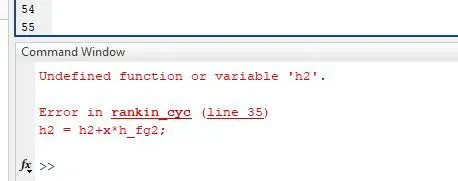
Undefined variable error.

Solution: The expression to calculate the enthalpy was wrongly defined, the expression is corrected to remove the error.

Error -2 (Similar type errors - 6)

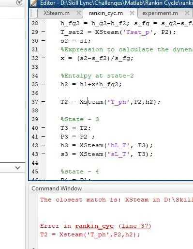
The 'Xstem' is undefined.

Solution: The function callout should be 'XSteam' instead of 'Xsteam'.

 Refrence:

1) https://www.youtube.com/watch?v=MQ13EepiG9Q

2)https://in.mathworks.com/help/physmod/simscape/ug/rankine-cycle-steam-turbine.html