Project 2 - Rankine cycle Simulator

clear all        % Clears the Workspace
close all        % Close all tabs
clc              % Clears the command window

%___________RANKINE CYCLE SIMULATOR - PROJECT____________%

% Process of Rankine cycle

fprintf('           RANKINE CYCLE SIMULATOR           \n');
fprintf('1-2 ISENTROPIC HEAT EXPANSION \n');
fprintf('2-3 CONSTANT PRESSURE HEAT REJECTION \n');
fprintf('3-4 ISENTROPIC COMPRESSION \n');
fprintf('4-1 CONSTANT PRESSURE HEAT ADDITION \n');

% Input values
T1 = input ('\n Turbine Inlet temperatute (in degree celcius) = ');
p1 = input (' Turbine Inlet Pressure (in bar) = ');
p2 = input (' Condensor Inlet Pressure (in bar) = ');

% State point-1 
h1 = XSteam('h_pT',p1,T1);    % Enthalphy at state point 1
s1 = XSteam('s_pT',p1,T1);    % Entropy at state point 1

% State point-2
s2 = s1;                    % Entropy at state point 2
sf2 = XSteam('sL_p',p2);
sg2 = XSteam('sV_p',p2);
x2 = (s2-sf2)/(sg2-sf2);
hf2 = XSteam('hL_p',p2);
hg2 = XSteam('hV_p',p2);
h2 = hf2+(x2*(hg2-hf2));    % Enthalphy at state point 2
T2 = XSteam('T_hs',h2,s2);  % Condensor outet Temperature 

% Work done by the Turbine (in KJ/Kg)
Wt = h1-h2;

% State point-3 
p3 = p2;                    % Pressure at Pump inlet
T3 = T2;                    % Temperature at Pump inlet
s3 = XSteam('sL_T',T3);     % Entropy at state point 3 
h3 = XSteam('hL_T',T3);     % Enthalphy at state point 3
v3 = XSteam('vL_p',p3);

% Heat Rejection in the Condensor (KJ)
Qr = h2-h3;

% State point-4
p4 = p1;                    % Pressure at boilerr inlet
s4 = s3;                    % Entropy at state point 4
Cp4 = XSteam('Cp_ps',p4,s4);
Cv4 = XSteam('Cv_ps',p4,s4);
gamma = Cp4/Cv4;
T4 = T3*(p4/p3)^(1-(1/gamma)); % Inlet temperature of the Bolier
% Work input to the Pump
% Wp = h4-h3 = v3(p4-p3)
Wp = v3*(p4-p3)*100;

% Then, h4 = Wp+h3
h4 = Wp+h3;                 % Enthalphy at state point 4

% Heat supplied to the Boiler
Qs = h1-h4;

% Net Work output
Wnet = Wt-Wp;

% Back Work Ratio
BWR = Wp/Wp;

% Efficiency of the cycle
E = (Wnet/Qs)*100;

% Steam flowrate per second
SSC = 3600/Wnet;

% State point-5
p5 = p1;                    % Pressure outlet at the Boiler
T5 = XSteam('Tsat_p',p5);   % Temperature outlet at the Bolier
s5 = XSteam('sL_p',p5);     % Entropy at statepoint point 5
h5 = XSteam('hL_p',p5);     % Enthalphy at state point 5

% State point-6
p6 = p5;
T6 = T5;
s6 = XSteam('sV_p',p6);     % Entropy at statepoint point 6
h6 = XSteam('hV_p',p6);     % Enthalphy at state point 6

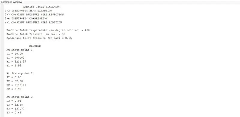
% Printing the results
fprintf('\n               RESULTS               \n');
fprintf(' At State point 1 \n P1 = %4.2f \n T1 = %4.2f \n H1 = %4.2f \n S1 = %4.2f \n\n',p1,T1,h1,s1);
fprintf(' At State point 2 \n P2 = %4.2f \n T2 = %4.2f \n H2 = %4.2f \n S2 = %4.2f \n\n',p2,T2,h2,s2);
fprintf(' At State point 3 \n P3 = %4.2f \n T3 = %4.2f \n H3 = %4.2f \n S3 = %4.2f \n\n',p3,T3,h3,s3);
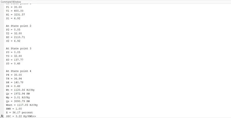
fprintf(' At State point 4 \n P4 = %4.2f \n T4 = %4.2f \n H4 = %4.2f \n S4 = %4.2f \n\n',p4,T4,h4,s4);
fprintf(' Wt = %4.2f KJ/Kg \n Qr = %4.2f KW \n Wp = %4.2f KJ/Kg \n Qs = %4.2f KW \n Wnet = %4.2f KJ/Kg \n BWR = %4.2f \n E = %4.2f percent \n SSC = %4.2f Kg/KWh',Wt,Qr,Wp,Qs,Wnet,BWR,E,SSC);

% Find T value
T = linspace(T6,T1,3000);
for i = 1:length(T)
    s(i) = XSteam('s_pT',p1,T(i));
end

% To plot Saturated liquid and vapour curve
T_curve = linspace(1,500,600);
for i = 1:length(T_curve)
    sf(i) = XSteam('sL_T',T_curve(i));
    sg(i) = XSteam('sV_T',T_curve(i));
    hf(i) = XSteam('hL_T',T_curve(i));
    hg(i) = XSteam('hV_T',T_curve(i));
end

% Plot for Temperature vs Entropy
figure (1);
plot([s1,s2,s3,s4,s5,s6,s],[T1,T2,T3,T4,T5,T6,T],'linewidth',2,'color','k');
text(s1,T1,'1');
text(s2,T2,'2');
text(s3,T3-20,'3');
text(s4,T4+30,'4');
text(s5,T5+20,'5');
text(s6-0.5,T6+30,'6');
hold on;
plot(sf,T_curve,'linewidth',1,'color','r');
plot(sg,T_curve,'linewidth',1,'color','b');
xlabel('Entropy (S) in KJ/K');
ylabel('Temperature (T) in degree C');
title('Temperature vs Entropy');
legend('T-S curve','Liquid Phase','Vapour Phase');

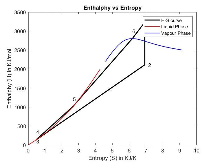
% Plot for Enthalphy vs Entropy
figure (2);
plot([s1,s2,s3,s4,s5,s6,s1],[h1,h2,h3,h4,h5,h6,h1],'linewidth',2,'color','k');
text(s1+0.2,h1,'1');
text(s2+0.2,h2,'2');
text(s3,h3-40,'3');
text(s4,h4+200,'4');
text(s5,h5+200,'5');
text(s6,h6+200,'6');
hold on;
plot(sf,hf,'linewidth',1,'color','r');
plot(sg,hg,'linewidth',1,'color','b');
xlabel('Entropy (S) in KJ/K');
ylabel('Enthalphy (H) in KJ/mol');
title('Enthalphy vs Entropy');
legend('H-S curve','Liquid Phase','Vapour Phase');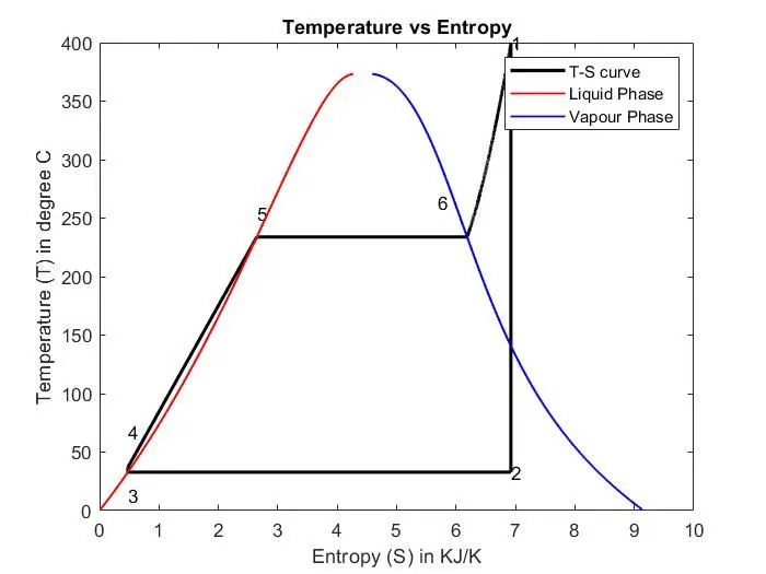

https://drive.google.com/file/d/1BOxz1OqYKg8DGOwHSa77f7ThP0Ovel3C/view?usp=drivesdk