Project 2 - Rankine cycle Simulator

AIM:

To write the program in Matalb for creating a Rankine Cycle Simulator.

OBJECTIVE:

• To calculate the state points of the Rankine Cycle based on the user inputs.
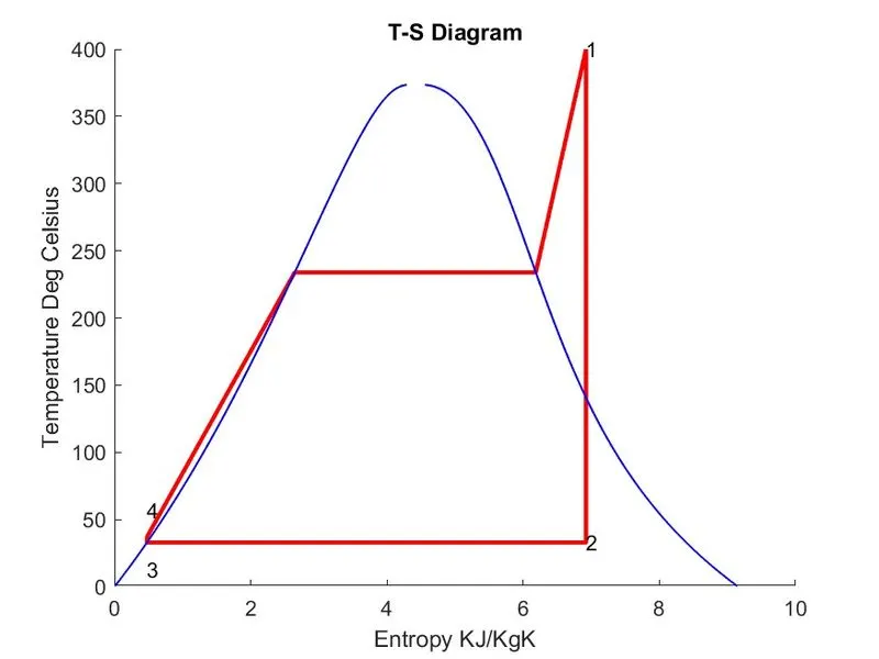
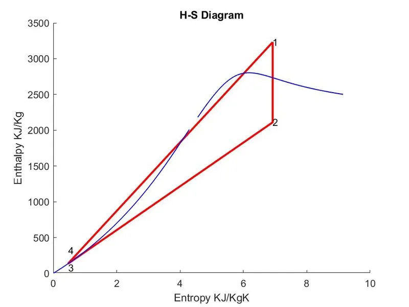
• To plot the corresponding T-s and h-s plots for the given set of inputs.

INTRODUCTION:

Rankine Cycle:

• The Rankine cycle is named after William John Macquorn Rankine, a Scottish polymath professor at Glasgow University. The Rankine Cycle describes the process of Stem engines which is commonly found in Thermal Power Generation Plants. The Rankine Cycle converts Thermal Energy into Mechanical Energy.
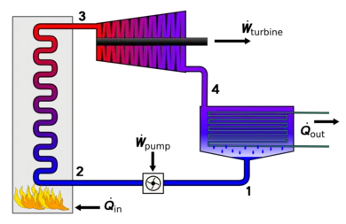
• The working of Rankine cycle is start with heating of water in boiler at constant pressure to produce steam. This steam is passed to the turbine and then isentropic expansion of steam takes place to produce work. Then the steam is moved to condenser and then the steam is cooled and converted into water at constant pressure. Then the water is pumped to the boiler using water pump and the cycle continues.

The Process of Rankine Cycle:

According to the above Image, the process are as follows:

• Process 1-2 - Isentropic Compression in Pump.The water is pumped from low to high pressure to Boiler.
• Process 2-3 - Constant Pressure Heat Addition in Boiler.: The high-pressure water enters the boiler and it is heated at constant pressure by an external heat source to become a dry saturated vapour or Steam.
• Process 3-4 - isentropic Expansion in Turbine.The dry saturated vapour or Steam gets expand in the turbine for generating the power. This decreases the temperature and pressure of the vapour or steam and also condensation may occur.
• Process 4-1 - Constant Pressure Heat Rejection in Condenser.The wet vapour or wet steam then enters into the condenser, where the wet vapour or wet steam is condensed at a constant pressure to become a saturated liquid.

The Formula For Calculating Efficiency, BWR, SSC:

• Dryness Fraction:

PROGRAM:

%Rankine Cycle Simulator

close all 
clear all
clc

%Description of Rankine Cycle and Printing the Description
fprintf ('      Rankine Cycle Simulatorn');
fprintf ('1-2 Isentropic Expansion in Turbinen');
fprintf ('2-3 Constant Pressure Heat Rejection in Condensern');
fprintf ('3-4 Isentropic Compression in the Pumpn');
fprintf ('4-1 Constant Pressure Heat Addition in Boilern');

%User Defining Inputs
fprintf('n');
P1 = input('Enter the Pressure at Turbine Inlet (in Bar) = ');
T1 = input('Enter the Temperature at Turbine Inlet (in Degree Celsius) = ');
P2 = input('Enter the Pressure at Turbine Outlet or Pressure at Condenser Inlet (in Bar) = ');

%Calculation of Saturation Temperture At P1 and P2
Tsat_P1 = XSteam('Tsat_P',P1);
Tsat_P2 = XSteam('Tsat_P',P2);

%Calculating Enthalpy and Entropy at Saturation State

%Calculating Saturation Properties at State 1
Hg_1 = XSteam('hV_p',P1);
Sg_1 = XSteam('sV_p',P1);

%Calculating Saturation Properties at State 2
Hg_2 = XSteam('hV_p',P2);
Sg_2 = XSteam('sV_p',P2);

%Calculating Saturation Properties at State 3
Hf_1 = XSteam('hL_p',P1);
Sf_1 = XSteam('sL_p',P1);

%Calculating Saturation Properties at State 4
Hf_2 = XSteam('hL_p',P2);
Sf_2 = XSteam('sL_p',P2);

%Calculating and Printing State Parameters

%At State 1
H1 = XSteam('h_pt',P1,T1);
S1 = XSteam('s_pt',P1,T1);

fprintf('n');
fprintf('At State Point 1n');
fprintf('P1 = %.2f Barn',P1);
fprintf('T1 = %.2f Deg Celsiusn',T1);
fprintf('H1 = %.2f KJ/Kgn',H1);
fprintf('S1 = %.2f Kj/KgKn',S1);

%At State 2
S2 = S1;                           %Since Isentropic Process
x = (S2-Sf_2)/(Sg_2-Sf_2);         %Dryness Fraction
T2 = Tsat_P2;
H2 = Hf_2 + x*(Hg_2-Hf_2);

fprintf('n');
fprintf('At State Point 2n');
fprintf('P2 = %.2f Barn',P2);
fprintf('T2 = %.2f Deg Celsiusn',T2);
fprintf('H2 = %.2f KJ/Kgn',H2);
fprintf('S2 = %.2f Kj/KgKn',S2);
fprintf('X = %.2f n',x);

%At State 3
P3 = P2;                           % Since Constant Pressure Process
V3 = XSteam('vL_p',P3);
T3 = Tsat_P2;
H3 = Hf_2;
S3 = Sf_2;

fprintf('n');
fprintf('At State Point 3n');
fprintf('P3 = %.2f Barn',P3);
fprintf('T3 = %.2f Deg Celsiusn',T3);
fprintf('H3 = %.2f KJ/Kgn',H3);
fprintf('S3 = %.2f Kj/KgKn',S3);

%At State 4
S4 = S3;                            %Since Isentropic Process
P4 = P1;
%Work Done by Pump,Wp = H4-H3 %H4-H3 = V3*(P4-P3)
Wp = V3*(P4-P3)*100;
H4 = H3+Wp;
Cp_4 = XSteam('Cp_ps',P4,S4);
Cv_4 = XSteam('Cv_ps',P4,S4);
k = Cp_4/Cv_4;
T4 = T3/((P3/P4)^((k-1)/k));

fprintf('n');
fprintf('At State Point 4n');
fprintf('P4 = %.2f Barn',P4);
fprintf('T4 = %.2f Deg Celsiusn',T4);
fprintf('H4 = %.2f KJ/Kgn',H4);
fprintf('S4 = %.2f Kj/KgKn',S4);

%Work Done By Turbine
Wt = H1-H2;
fprintf('n');
fprintf('Work Done by Turbine Wt  = %.2f KJ/Kgn',Wt);

%Work Done By Pump
fprintf('Work Done by Pump Wp  = %.2f KJ/Kgn',Wp);

%Net Work Done
Wnet = Wt-Wp;
fprintf('Net Work Done Wnet  = %.2f KJ/Kgn',Wnet);

%Heat Added
Q_add = H1-H4;

%Heat Rehected
Q_rej = H2-H3;

%Thermal Efficiency
N_Thermal = (Wnet/Q_add)*100;
fprintf('Thermal Efficiency = %.2f percentn',N_Thermal);

%Specific Steam Consumption
SSC = 3600/Wnet;
fprintf('Specific Steam Consumption SSC = %.2f Kg/KWhn',SSC);

%Back Work Ratio
BWR = Wp/Wt;
fprintf('Back Work Ratio BWR = %.3f n',BWR);

%Plotting T-S and H-S Saturation Curves

%Defining the Temperature Range for Saturation Curves
T = linspace(0,T1,1000);
for i = 1:length(T)
    hL (i) = XSteam('hL_T',T(i));
    hV (i) = XSteam('hV_T',T(i));
    sL (i) = XSteam('sL_T',T(i));
    sV (i) = XSteam('sV_T',T(i));
end

%Plotting T-S Curve
figure(1)
hold on
plot([S1 S2 S3 S4 Sf_1 Sg_1 S1],[T1 T2 T3 T4 Tsat_P1 Tsat_P1 T1],'LineWidth',2,'Color','r')
plot(sL,T,'Linestyle','-','LineWidth',1,'Color','b')
plot(sV,T,'Linestyle','-','LineWidth',1,'Color','b') 
text (S1,T1,'1')
text (S2,T2,'2')
text (S3,T3-20,'3')
text (S4,T4+20,'4')

title('T-S Diagram')
xlabel ('Entropy KJ/KgK')
ylabel ('Temperature Deg Celsius')
saveas(figure(1),'T-S Diagram.jpg')

%Plotting H-S Curve
figure(2)
hold on
plot([S1 S2 S3 S4 S1],[H1 H2 H3 H4 H1],'LineWidth',2,'Color','r')
plot(sL,hL,'Linestyle','-','LineWidth',1,'Color','b')
plot(sV,hV,'Linestyle','-','LineWidth',1,'Color','b')
text (S1,H1,'1')
text (S2,H2,'2')
text (S3,H3-60,'3')
text (S4,H4+180,'4')

title('H-S Diagram')
xlabel ('Entropy KJ/KgK')
ylabel ('Enthalpy KJ/Kg')
saveas(figure(2),'H-S Diagram.jpg')

• First we start with Close all, Clear all and clc before start of program,because Close all - deletes the current figures or thespecified figures, Clear all - deletes the data from workspace and clear the system memory and clc - clear the data present in the Command Window and gives clean Command Window.
• The 'fprintf' command is used for display the Rankine cycle and their Process 1-2 Isentropic Expansion in Turbine, 2-3 Constant Pressure Heat Rejection in Condenser, 3-4 Isentropic Compression in the Pump, 4-1 Constant Pressure Heat Addition in Boiler in the command window.
• The'n' command is used for inserting new line for a character in command window.
• The 'input()' command is used to define the user inputs, by using this command the Pressure at Turbine Inlet (P1), Temperature at Turbine Inlet (T1), Pressure at Turbine Outlet or Pressure at Condenser Inlet (P2) the input is defined by user in command window and they are assigned to P1, T1 and P2 variables respectively.
• The Saturation Temperature for P1 and P2 is calculated using 'XSteam()' function that is the steam table Matlab program. This function program consits of all thrmodynamics properties.By calling the function the thermodynamic property will be provided based on the parameters such as pressure, temperature,etc. In this Saturation temperature is found based on the pressure and it is assigned to Tsat_P1 and Tsat_P2 respectively.
• The Enthalpy and Entropy for liquid and vapour at saturation state at 1,2,3 and 4 are found out using 'Xsteam()' function based on the pressure P1 and P2 and assigned to variables Hg_1, Sg_1, Hg_2, Sg_2, Hf_1, Sf_1,Hf_2, Sf_2.
• The state 1 parameters Enthalpy (H1) and Entropy (S1),P1, T1 are calculated using 'Xsteam()' function and 'fprintf' is used for displying the output in the command window and '%.2f' is used for displaying the only 2 decimal values after the decimal point and the'n' command is used for inserting new line for a character in command window.
• The state 2 parameters Dryness Fraction (x) and Enthalpy (H2),S2,P2,T2 using Dryness Fraction are calculated and 'fprintf' is used for displying the output in the command window and '%.2f' is used for displaying the only 2 decimal values after the decimal point and the'n' command is used for inserting new line for a character in command window. Likewise state 3 H3,P3,T3,S3 and state 4 H4,T4,P4,S4 parameters are calculated and displayed in the command window.
• Using all these four state parameters the Work Done by Turbine, Work Done by Pump, Net Work Done, Thermal Efficiency, SSC, Bwr are calculated using above mentioned formulas and 'fprintf' is used for displying the output in the command window and '%.2f' is used for displaying the only 2 decimal values after the decimal point and the'n' command is used for inserting new line for a character in command window.
• The 'For' Loop is used for calculating the saturation curve of enthalpy and entropy for temperature range from 0 to T1 upto 1000 values using 'Linspace' command for creating evenly spaced elements, it is assigned to T variable and the entropy and enthalpy assigned to variables hl,hv,sl,sv .
• The 'Figure(1)' command is used to create the figure graphical object.
• The 'Plot' command is used for plotting the T-S plot that is entropy [S1 S2 S3 S4 Sf_1 Sg_1 S1] vs temperature [T1 T2 T3 T4 Tsat_P1 Tsat_P1 T1] and 'Linewidth' command is used for thicker line in the graph of width 2 is used to show thicker line and 'Color' command is used with 'r' for red color line.
• The 'Plot' command is used for plotting the entropy sl and sv calculated using for loop vs temperature range T and 'Linestyle' command is used for creating the types of line style to be displayed in the plot and '-' is used for - line in the plot 'Linewidth' command is used for thicker line in the graph of width 1 is used to show thicker line and 'Color' command is used with 'b' for blue color line.
• The 'xlabel ('Entropy KJ/KgK')' is mentioned to show x-axis as Entropy KJ/KgK in the graph and'ylabel ('Temperature Deg Celsius')' command is used to y-axis as Temperature Deg Celsius in the graph.
• The 'Title' command is used for giving title of graph and the title is T-S Diagram.
• The 'text' command is used for adding the description text to the plot and in this (S1,T1,'1') to display 1 to S1 and T1.
• The 'text' command is used for adding the description text to the plot and in this (S2,T2,'2') to display 2 to S2 and T2.
• The 'text' command is used for adding the description text to the plot and in this (S3,T3-20,'3') to display 3 to S3 and T3 before 20 values to avoid overlapping with the plot.
• The 'text' command is used for adding the description text to the plot and in this (S4,T4+20,'4') to display 4 to S4 and T4 after 20 values to avoid overlapping with the plot.
• The 'Saveas' command is used to save all there plots as figure(1) as T-S Diagram.
• The 'Figure(2)' command is used to create the figure graphical object.
• The 'Plot' command is used for plotting the H-S plot that is entropy [S1 S2 S3 S4 S1] vs enthalpy [H1 H2 H3 H4 H1] and 'Linewidth' command is used for thicker line in the graph of width 2 is used to show thicker line and 'Color' command is used with 'r' for red color line.
• The 'Plot' command is used for plotting the entropy sl and sv vs enthalpy hl and hv respectively calculated using for loop and 'Linestyle' command is used for creating the types of line style to be displayed in the plot and '-' is used for - line in the plot 'Linewidth' command is used for thicker line in the graph of width 1 is used to show thicker line and 'Color' command is used with 'b' for blue color line.
• The 'xlabel ('Entropy KJ/KgK')' is mentioned to show x-axis as Entropy KJ/KgK in the graph and'ylabel ('Enthalpy KJ/Kg')' command is used to y-axis as Enthalpy KJ/Kg' in the graph.
• The 'Title' command is used for giving title of graph and the title is H-S Diagram.
• The 'text' command is used for adding the description text to the plot and in this (S1,H1,'1') to display 1 to S1 and H1.
• The 'text' command is used for adding the description text to the plot and in this (S2,H2,'2') to display 2 to S2 and H2.
• The 'text' command is used for adding the description text to the plot and in this (S3,H3-60,'3') to display 3 to S3 and H3 before 60 values to avoid overlapping with the plot.
• The 'text' command is used for adding the description text to the plot and in this (S4,H4+180,'4') to display 4 to S4 and H4 after 180 values to avoid overlapping with the plot.
• The 'Saveas' command is used to save all there plots as figure(2) as H-S Diagram.

OUTPUT:
T-S Diagram:

H-S Diagram:

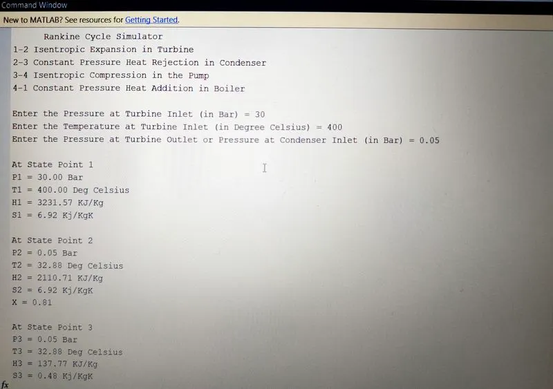
Results in Command Window:

Rankine Cycle Simulator
1-2 Isentropic Expansion in Turbine
2-3 Constant Pressure Heat Rejection in Condenser
3-4 Isentropic Compression in the Pump
4-1 Constant Pressure Heat Addition in Boiler

Enter the Pressure at Turbine Inlet (in Bar) = 30
Enter the Temperature at Turbine Inlet (in Degree Celsius) = 400
Enter the Pressure at Turbine Outlet or Pressure at Condenser Inlet (in Bar) = 0.05

At State Point 1
P1 = 30.00 Bar
T1 = 400.00 Deg Celsius
H1 = 3231.57 KJ/Kg
S1 = 6.92 Kj/KgK

At State Point 2
P2 = 0.05 Bar
T2 = 32.88 Deg Celsius
H2 = 2110.71 KJ/Kg
S2 = 6.92 Kj/KgK
X = 0.81

At State Point 3
P3 = 0.05 Bar
T3 = 32.88 Deg Celsius
H3 = 137.77 KJ/Kg
S3 = 0.48 Kj/KgK

At State Point 4
P4 = 30.00 Bar
T4 = 36.94 Deg Celsius
H4 = 140.78 KJ/Kg
S4 = 0.48 Kj/KgK

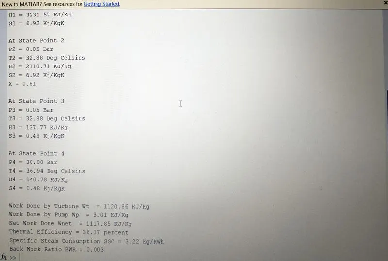
Work Done by Turbine Wt = 1120.86 KJ/Kg
Work Done by Pump Wp = 3.01 KJ/Kg
Net Work Done Wnet = 1117.85 KJ/Kg
Thermal Efficiency = 36.17 percent
Specific Steam Consumption SSC = 3.22 Kg/KWh
Back Work Ratio BWR = 0.003

Screenshot of Results in Command Window:

ERROR fACED WHILE PROGRAMMING:
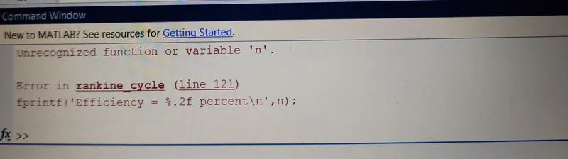
Typo error, I assigned variable for the thermal efficiency as N_Thermal, But while using the fprintf command for displaying the efficiency i mentioned the efficiency variable as n. So the command window throws an error as unrecognized function or variable 'n'.

Screenshot showing errors thrown in command window:

Steps taken to overcome those errors:

Now I correctly mentioned the efficiency variable N_Thermal and now the program run successfully without throwing any error.

CONCLUSION:

Thus the program is written in Matlab for a Rankine Cycle Simulation and also calculated the state points of the Rankine Cycle based on the user inputs and also ploted the corresponding T-s and h-s plots for the given set of inputs.

REFERENCE:

• www.nuclear-power.com/nuclear-engineering/thermodynamics/thermodynamic-cycles/rankine-cycle-steam-turbine-cycle/theory-of-rankine-cycle-equations-and-calculation/
• www.nuclear-power.com/nuclear-engineering/thermodynamics/thermodynamic-cycles/rankine-cycle-steam-turbine-cycle/superheat-and-reheat-rankine-cycle/
• n.mathworks.com/help/matlab/ref/input.html
• https://in.mathworks.com/help/matlab/matlab_prog/formatting-strings.html