Air standard Cycle
Aim:
To write the program to calculate thermal efficiency for Otto Cycle and make plots for Otto Cycle using Matlab.
Intoduction:
The Otto Cycle:
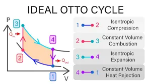
Otto Cycle Process based on the above image are as follows:
- Process 1-2: It is Isentropic (Adiabatic) Compression process. In this process the piston moves from Bottom Dead Centre to Top Dead Centre forn compressing the working fluid.
- Process 2-3: It is Constant Volume Heat addition process. In this process the heat transferd from external source to working fluid while piston at Top Dead Centre that is the ignition of air-fuel mixture takes place and rapid burning occurs.
- Process 3-4: It is an Isentropic (Adiabatic) Expansion. In this process the the piston moves from Top Dead Centre to Bottom Dead Centre and completes expansion process. It is also called as Power Stroke.
- Process 4-1: It is Constant Volume Heat Rejection process. In this process heat is rejected from air while piston at Bottom Dead Centre.
To Solve Otto Cycle:
In this program we use Engine Geometrics. The Engine Geometric parameters are:
- Bore = 0.3 m;
- Stroke = 0.1 m;
- Connecting Rod (con_rod) = 0.16 m;
- Compression Ratio (cr) = 8;
The Inputs for State Variables are as follows:
- p1 = 101325 Pa;
- t1 = 500 K;
- gamma = 1.5;
- t3 = 2400 K;
The Formula Used To Calcluate Otto Cycle Process:
- Swept Volume :
- Clearance Volume:
v_clearance = v_swept / (cr-1)
- Isentropic Process:
P*V^gamma = Constant
- Combined Gas Law:
(P*V)/T = Constant
- Volume Trace or Volume Compression or Expansion:
- Thermal efficiency
thermal_efficiency = (1-(1/cr^(gamma-1)))*100
% To Calculate the Thermal Efficiency of Otto Cycle and Plot the Otto Cycle

close all
clear all
clc

% Inputs

% State Variables
p1 = 101325; % in Pascal
t1 = 500; % in Kelvin
gamma = 1.5;
t3 = 2400; % in Kelvin

% Engine Geometric Parameters
bore = 0.3;
stroke = 0.1;
con_rod = 0.16;
cr = 8;

% Calculating Swept Volume and Clearance Volume
v_swept = (pi/4)*bore^2*stroke;
v_clearance = v_swept / (cr-1);
v1 = v_swept + v_clearance;
v2 = v_clearance;

% State Variables at State Point 2
%p2*v2^gamma = p1*v1^gamma | p2 = p1 *(v2/v1)^gamma | p2 = p1*cr^ gamma
p2 = p1*cr^gamma;

%(p1*v1)/t1=(p2*v2)/t2 | t2 =(p2*v2*t1)/(p1*v1)
t2 =(p2*v2*t1)/(p1*v1);

constant1 = p1*v1^gamma;
V_compression = engine_kinematics(bore,stroke,con_rod,cr,180,0);
P_compression = constant1./(V_compression.^gamma);

% State Variables at State Point 3
v3 = v2;
%(p3*v3)/t3 = (p2*v2)/t2 | p3 =(p2*t3)/t2
p3 =(p2*t3)/t2;

constant2 = p3*v3^gamma;
V_expansion = engine_kinematics(bore,stroke,con_rod,cr,0,180);
P_expansion = constant2./(V_expansion.^gamma);

% State Variables at State Point 4
v4 = v1;
%p3*v3^gamma = p4*v4^gamma | p4 = p13 *(v3/v4)^gamma
p4 = p3 *(v3/v4)^gamma;

% Thermal efficiency
thermal_efficiency = (1-(1/cr^(gamma-1)))*100

% Plotting Otto Cycle
figure(1)
hold on
plot ([v2,v3], [p2,p3], 'LineWidth',1, 'Color','r')
plot (V_compression,P_compression, 'LineWidth',1, 'Color','b')
plot (V_expansion,P_expansion, 'LineWidth',1, 'Color','g')
plot ([v4,v1], [p4,p1], 'LineWidth',1, 'Color','m')
xlabel ('Volume')
ylabel ('Pressure')
axis ([0 0.009 0 4*10^6])
grid on- The Inputs of the State variables such as p1,t1,gamma, t3 and Engine Geometric parameters such as bore, stroke, connecting rod, compression ratio are assigned as mentioned above in the program.
- The swept volume, v_swept and clearance volume, v_clearance are calculated using swept volume and clearance formula and also volume at state pont 1, v1 and volume at state pont 2, v2 are calculated using swept volume and clearance volume.
- The state variable at state ponit 2 pressure, p2 is calculated using Isentropic formula.
- The constant1 value is calculated using Isentropic formula to calculate Pressure at compression state.
- The Volume at compression state is calculated by calling the function engine_kinemattics.The Call of Function is used to invoke the function by just mentioning the function name and input arguments.By specifing the function name and their inputs the function will be called of and runs the function program. In this program the functiuon name is engine_kinematics and the inputs are bore,stroke,con_rod,cr,start_crank,end_crank and these are mentioned in the Code of Function for Piston Kinematics which the program written in seperate window.The element wise operator since the theta is matrix of 1x100
- The Pressure at compression is calculated by using Isentropic formula. The element wise operator since the Volume at compression is matrix of 1x100
- The state variable at state ponit 3 volume 3 is equal to volume 2 as this process in constant volume process that is v2 = v3.
- The state variable at state ponit 3 pressure, p3 is calculated using Combined Gas Law.
- The constant2 value is calculated using Isentropic formula to calculate Pressure at expansion state.
- The Volume at expansion state is calculated by calling the function engine_kinemattics.The Call of Function is used to invoke the function by just mentioning the function name and input arguments.By specifing the function name and their inputs the function will be called of and runs the function program. In this program the functiuon name is engine_kinematics and the inputs are bore,stroke,con_rod,cr,start_crank,end_crank and these are mentioned in the Code of Function for Piston Kinematics which the program written in seperate window.The element wise operator since the theta is matrix of 1x100.
- The Pressure at expansion is calculated by using Isentropic formula.The element wise operator since the Volume at expansion is matrix of 1x100
- The state variable at state ponit 4 pressure, p4 is calculated using Isentropic formula.
- The Thermal efficiency is calculated using thermal efficiency formula.
- The 'Plot' command is used to create the plot between ([v2 v3],[p2 p3]), the 'Linewidth' command is used for thicker line of width 1,the 'Color' command is used to color the line of 'r' command which means red color line is used for plotting.
- The 'Plot' command is used to create the plot between (V_compression,P_compression), the 'Linewidth' command is used for thicker line of width 1,the 'Color' command is used to color the line of 'b' command which means blue color line is used for plotting.
- The 'Plot' command is used to create the plot between (V_expansion,P_expansion), the 'Linewidth' command is used for thicker line of width 1,the 'Color' command is used to color the line of 'g' command which means green color line is used for plotting.
- The 'Plot' command is used to create the plot between ([v4 v1],[p4 p1]), the 'Linewidth' command is used for thicker line of width 1,the 'Color' command is used to color the line of 'm' command which means magenta color line is used for plotting.
- The 'Figure(1)' command is used to create the figure graphical object.
- The 'Hold on' command is used for second line plot without deleting the existing line plot.
- The 'axis' command is used to set the limit for x-axis and y-axis.In this program the limit is set by 0 to 0.009 for x-axis and 0 to 4*10^6 for y-axis.
- The "xlabel ('Volume')" is mentioned to show x-axis as Volume in the graph and "ylabel (Pressure)" command is used to y-axis as Pressure in the graph.
- The "grid on" command is used to show the grids in the graph.
Code of Function for Piston Kinematics :
function [V] = engine_kinematics (bore,stroke,con_rod,cr,start_crank,end_crank)

a = stroke/2;
R = con_rod/a;

v_swept = (pi/4)*bore^2*stroke;
v_clearance = v_swept/(cr-1);

theta = linspace(start_crank,end_crank,100);

term1 = 0.5*(cr-1);
term2 = R+1-cosd(theta);
term3 = (R^2-sind(theta).^2).^0.5;

V = (1+term1*(term2-term3)).*v_clearance;

end- The function code is used for calculate the trace volume using piston kinematics.
- The function should contain function keyword followed by input arguments then the function name and folllowed by the output arguments In this program the function is defined as function [V] = engine_kinematics (bore, stroke,con_rod,cr,start_crank,end_crank) where function is the function keyword, [V] is input arguments, engine_kinematics is function name and bore, stroke,con_rod,cr,start_crank,end_crank are output arguments.
- The file name stored and function name used in function definition should be same otherwise the program throws an error.
- The Function should contain input argument and the input which is to provided by user should match exact number of input arguments provided in the function definition .In this program the input arguments are bore,stroke,con_rod,cr,start_crank,end_crank, the user should provide values for these inputs if not provided it shows error msessage that the input missing varialbe is not defined.
- Likerwise the output arguments should match the output variables defined in the function definition. In this program V is used as output arguments and it is also defined in the program.
- The theta values uses 'Linspace ' command to obtain evenly sapced elements.
- The a and R values are calculated.
- The swept volume, v_swept and clearance volume, v_clearance are calculated using swept volume and clearance formula
- The Volume trace is calculted using the volume trace formula.The element wise operator since the theta is matrix of 1x100
- The volume trace formula is seperated into three terms.
- These three terms combined for calculating the trace volume.
- The 'end' command is used to stop the function running.
Error faced while progrming is:
I had not use element wise operator to the constant2 as the V_expansion is the matrix of 1x100 while calculating the pressure at expansion state that is P_expansion = contant2/(V_expansion.^gamma). The command window shows an error that is matrix dimension should agree.
Screen shot of the error displayed in the Command Window:
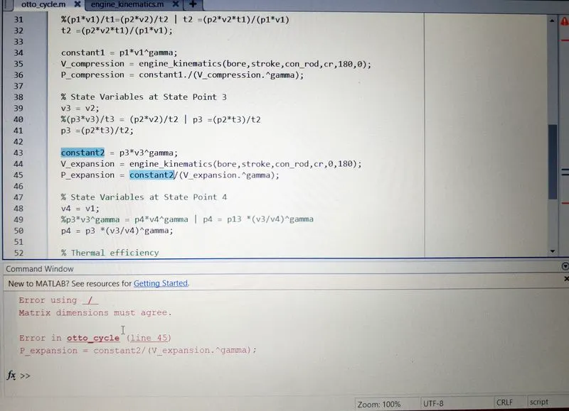
Steps taken to overcome those errors:
After using element wise operator to the constant2 while calculating the pressure at expansion state that is P_expansion = contant2/(V_expansion.^gamma) the program runs without any error.
Output:
Thermal Efficiency:
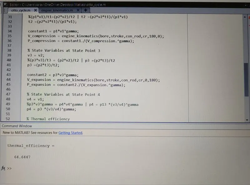
The Thermal efficiency of the Otto Cycle is 64.6447%
Plotting PV Diagram:
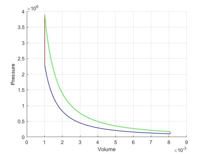
Thus the result shows that when compression ratio is high the thermal efficiency is also high.
Conclusion:
Thus the program is written to calculate the thermal efficiency for Otto Cycle and PV diagram is obtained for Otto Cycle using Matlab.