Challenge

Project 2 - Rankine cycle Simulator

AAltrin Rijo18 May 2022

Rankine cycle stimulator using MATLAb

Aim:-

To stimulate the Rankine cycle using the matlab and to find out the parameters like Pressure, temperature, enthalpy & entropy at all the for state points and also to find out the Net work and back work ratio. After attaing all the state points, they are plotted and Ts & Pv diagrams are generated.

Software used:-

MATLAB R2022a

Project Description:-

Rankine cycle:-

The Rankine cycle is an idealized thermodynamic cycle describing the process by which certain heat engines, such as steam turbines or reciprocating steam engines, allow mechanical work to be extracted from a fluid as it moves between a heat source and heat sink.

Heat energy is supplied to the system via a boiler where the working fluid (typically water) is converted to a high pressure gaseous state (steam) in order to turn a turbine. After passing over the turbine the fluid is allowed to condense back into a liquid state as waste heat energy is rejected before being returned to boiler, completing the cycle.

Processes in Rankine cycle:-

The Rankine cycle is the ideal cycle for vapor power plants; it includes the following four
reversible processes:

Process 1–2 Isentropic Expansion: The dry saturated vapour expands through a turbine, generating power. This decreases the temperature and pressure of the vapour, and some condensation may occur.

Process 2–3 Constant pressure heat rejection: The wet vapour then enters a condenser, where it is condensed at a constant pressure to become a saturated liquid.

Process 3–4 Isentropic Compression: The working fluid is pumped from low to high pressure. As the fluid is a liquid at this stage, the pump requires little input energy.

Process 4–1 Constant pressure heat addition: The high-pressure liquid enters a boiler, where it is heated at constant pressure by an external heat source to become a dry saturated vapour.

These process can be explained with the help of the following diagram:-

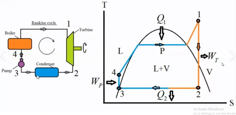
Now here in our project, we will try to find out Pressure, temperature, entropy and enthalpy for all the state points and also will find out the parameters like net work done and back work ratio for the given inputs.

Program with Explainations:-

clear all

close all

clc

%Given inputs

T1=300;

P1=20;

P4=P1;

P2=0.07;

P3=P2;

In the above code, the input parameters are assigned to the respective variables.

At state point 1:-

%Calculating entropy and enthalpy at point 1

h1=XSteam('h_pT',P1,T1);

s1=XSteam('s_pT',P1,T1);

Since the T1 & P1 are already defined, the h1 & s1 values are taken from the XSteam library provided.

'h_pT' & 's_pT'= Enthalpy & Entropy at particular pressure and temperature ( The values will be taken from the XSteam library from the matlab)

At state point 2:-

%At state point 2

s2=s1;

%For an isentropic expansion, ( T2/T1 )= (P2/P1)^(1-(1/gamma))

gamma=1.4;

power=(1-(1/gamma));

T2=T1*((P2/P1)^power);

h2=XSteam('h_pT',P2,T2);

Then for the state point 2, all the unknown parameters are calculated. T2 is calculated from the isentropic expansion relation, since at state point to expansion occurs.

At state point 3:-

%At state point 3

T3=T2;

h3=XSteam('hL_T',T3);

s3=XSteam('sL_T',T3);

Similarly at state point 3 all the values are calculated as mentioned above. Here , 'hL_T' & 'sL_T' represents, the entropy and enthalpy at liquid state fro the attained temperature.

At state point 4:-

%At state points 4

s4=s3;

T4=XSteam('T_ps',P4,s4);

h4=XSteam('h_pT',P4,T4);

h41=XSteam('hL_p',P4);

s41=XSteam('sL_p',P4);

h42=XSteam('hV_p',P4);

s42=XSteam('sV_p',P4);

T41=XSteam('T_hs',h41,s41);

T42=XSteam('T_hs',h42,s42);

The same procedure is repeated and all the respective points at state 4 have been calculated, depending upon the state of the liquid.

To calculate the Work done by the turbine, pump & net work done:-

%To calculate the net work output

w_t=h1-h2;

w_p=h4-h3;

w_net=w_t-w_p;

Here, w_t = Work done by the turbine

w_p= Work done to the Pump

w_net= Net work done

To calculate the other parameters:-

%To calculate back work ratio

bwr=w_p/w_t;

%To calculate Heat supplied & Heat rejected

qs=h1-h4

qr=h2-h3

%To calculate thermal efficiency

thermal_eff=(w_net/qs)*100;

%To calculate specific steam consumption

ssc=3600/w_net;

Now the other parameters Back work ratio(bwr) , Heat supplied (qs) , Heat rejected (qr), Thermal efficiency (thermal_eff), Specific steam consumption (ssc) have been calculated by the help of the above code.

To create the doom curve for all the entropy and enthalpy at liquid and vapour conditions:-

%To calculate enthalpy and entropy values to get the whole curve

temp=linspace(1,500,600)

for i=1:length(temp)

sl(i)=XSteam('sL_T',temp(i))

sv(i)=XSteam('sV_T',temp(i))

hl(i)=XSteam('hL_T',temp(i))

hv(i)=XSteam('hV_T',temp(i))

end

By the help of the above code the enthalpy and entropy at the liquid and vapour states are calculated .

%Plotting

figure(1);

plot([s1 s2],[T1 T2],[s2 s3],[T2 T3],[s3 s4],[T3 T4],[s4 s41],[T4 T41],[s41 s42],[T41 T42],[s42 s1],[T42 T1],'marker','*','color','r')

hold on

plot(sl,temp)

plot(sv,temp)

xlabel('Entropy (KJ/Kg K)');

ylabel('Temperature (K)');

Now from the above code, the plotting has been done for all the entropy and temperature ( TS diagram ) and has been plotted.

figure(2)

plot([s1 s2],[h1 h2],[s2 s3],[h2 h3],[s3 s4],[h3 h4],[s4 s1],[h4 h1],'marker','*','Color','g')

hold on

plot(sv,hv);

plot(sl,hl);

xlabel('Entropy (KJ/KgK)')

ylabel('Enthalpy (KJ/K)')

Now from the above code, the plotting has been done for all the entropy and enthalpy ( HS diagram ) and has been plotted.

%Displaying the results

disp('Results');

disp('Given inputs');

P1=P1

P2=P2

T1=T1

disp('At state point 1');

n1=sprintf('P1 is %.3f bar',P1);

disp(n1);

n2=sprintf('T1 is %.3f degree celcius',T1);

disp(n2);

n3=sprintf('h1 is %.3f KJ/Kg',h1);

disp(n3);

n4=sprintf('s1 is %.3f KJ/KgK',s1);

disp(n4);

disp('At state point 2');

n5=sprintf('P2 is %.3f bar',P2);

disp(n5);

n6=sprintf('T2 is %.3f degree celcius',T2);

disp(n6);

n7=sprintf('h2 is %.3f KJ/Kg',h2);

disp(n7);

n8=sprintf('s2 is %.3f KJ/KgK',s2);

disp(n8);

disp('At state point 3');

n9=sprintf('P3 is %.3f bar',P3);

disp(n9);

n10=sprintf('T3 is %.3f degree celcius',T3);

disp(n10);

n11=sprintf('h3 is %.3f KJ/Kg',h3);

disp(n11);

n12=sprintf('s3 is %.3f KJ/KgK',s3);

disp(n12);

disp('At state point 4');

n13=sprintf('P3 is %.3f bar',P4);

disp(n13);

n14=sprintf('T4 is %.3f degree celcius',T4);

disp(n14);

n15=sprintf('h4 is %.3f KJ/Kg',h4);

disp(n15);

n16=sprintf('s4 is %.3f KJ/KgK',s4);

disp(n16);

disp('calculated parameters');

n17=sprintf('Work done by the turbine = %.3f',w_t);

disp(n17);

n18=sprintf('Work done by the pump = %.3f',w_p);

disp(n18);

n19=sprintf('Heat supplied = %.3f KJ/K',qs);

disp(n19);

n20=sprintf('Heat rejected = %.3f KJ/K',qr);

disp(n20);

n21=sprintf('Net work done = %.3f KJ/K',w_net);

disp(n21);

n22=sprintf('Thermal efficiency = %.3f %',thermal_eff);

disp(n22);

n23=sprintf('Specific Steam consumption(ssc) = %.3f Kg/KW h',ssc);

disp(n23);

n24=sprintf('Back Work ratio = %.3f',bwr);

disp(n24);

Now all the calculated values are displayed in the command window. 'sprintf' code is used to print the values '%.3f' is used to print the values with three decimal points

All the lines are stored in seperate lines as ( n1,n2,....n24) and are indiviually displayed.

Program:-

clear all
close all
clc

%Given inputs

T1=300;
P1=20;
P4=P1;
P2=0.07;
P3=P2;

%Calculating entropy and enthalpy at point 1

h1=XSteam('h_pT',P1,T1);
s1=XSteam('s_pT',P1,T1);

%At state point 2

s2=s1;

%For an isentropic expansion, ( T2/T1 )= (P2/P1)^(1-(1/gamma))
gamma=1.4;
power=(1-(1/gamma));
T2=T1*((P2/P1)^power);
h2=XSteam('h_pT',P2,T2);

%At state point 3

T3=T2;
h3=XSteam('hL_T',T3);
s3=XSteam('sL_T',T3);

%At state points 4

s4=s3;
T4=XSteam('T_ps',P4,s4);
h4=XSteam('h_pT',P4,T4);
h41=XSteam('hL_p',P4);
s41=XSteam('sL_p',P4);
h42=XSteam('hV_p',P4);
s42=XSteam('sV_p',P4);
T41=XSteam('T_hs',h41,s41);
T42=XSteam('T_hs',h42,s42);

%To calculate the net work output

w_t=h1-h2;
w_p=h4-h3;
w_net=w_t-w_p;

%To calculate back work ratio

bwr=w_p/w_t;

%To calculate Heat supplied & Heat rejected

qs=h1-h4
qr=h2-h3

%To calculate thermal efficiency

thermal_eff=(w_net/qs)*100;

%To calculate specific steam consumption

ssc=3600/w_net;

%To calculate enthalpy and entropy values to get the whole curve

temp=linspace(1,500,600)
for i=1:length(temp)

    sl(i)=XSteam('sL_T',temp(i))
    sv(i)=XSteam('sV_T',temp(i))

    hl(i)=XSteam('hL_T',temp(i))
    hv(i)=XSteam('hV_T',temp(i))
 
end

%Plotting

figure(1);
plot([s1 s2],[T1 T2],[s2 s3],[T2 T3],[s3 s4],[T3 T4],[s4 s41],[T4 T41],[s41 s42],[T41 T42],[s42 s1],[T42 T1],'marker','*','color','r')
hold on
plot(sl,temp)
plot(sv,temp)
xlabel('Entropy (KJ/Kg K)');
ylabel('Temperature (K)');

figure(2)
plot([s1 s2],[h1 h2],[s2 s3],[h2 h3],[s3 s4],[h3 h4],[s4 s1],[h4 h1],'marker','*','Color','g')
hold on
plot(sv,hv);
plot(sl,hl);
xlabel('Entropy (KJ/KgK)')
ylabel('Enthalpy (KJ/K)')

%Displaying the results

disp('Results');
disp('Given inputs');
P1=P1
P2=P2
T1=T1

disp('At state point 1');
n1=sprintf('P1 is %.3f bar',P1);
disp(n1);
n2=sprintf('T1 is %.3f degree celcius',T1);
disp(n2);
n3=sprintf('h1 is %.3f KJ/Kg',h1);
disp(n3);
n4=sprintf('s1 is %.3f KJ/KgK',s1);
disp(n4);

disp('At state point 2');
n5=sprintf('P2 is %.3f bar',P2);
disp(n5);
n6=sprintf('T2 is %.3f degree celcius',T2);
disp(n6);
n7=sprintf('h2 is %.3f KJ/Kg',h2);
disp(n7);
n8=sprintf('s2 is %.3f KJ/KgK',s2);
disp(n8);

disp('At state point 3');
n9=sprintf('P3 is %.3f bar',P3);
disp(n9);
n10=sprintf('T3 is %.3f degree celcius',T3);
disp(n10);
n11=sprintf('h3 is %.3f KJ/Kg',h3);
disp(n11);
n12=sprintf('s3 is %.3f KJ/KgK',s3);
disp(n12);

disp('At state point 4');
n13=sprintf('P3 is %.3f bar',P4);
disp(n13);
n14=sprintf('T4 is %.3f degree celcius',T4);
disp(n14);
n15=sprintf('h4 is %.3f KJ/Kg',h4);
disp(n15);
n16=sprintf('s4 is %.3f KJ/KgK',s4);
disp(n16);

disp('calculated parameters');
n17=sprintf('Work done by the turbine = %.3f',w_t);
disp(n17);
n18=sprintf('Work done by the pump = %.3f',w_p);
disp(n18);
n19=sprintf('Heat supplied = %.3f KJ/K',qs);
disp(n19);
n20=sprintf('Heat rejected = %.3f KJ/K',qr);
disp(n20);
n21=sprintf('Net work done = %.3f KJ/K',w_net);
disp(n21);
n22=sprintf('Thermal efficiency = %.3f %',thermal_eff);
disp(n22);
n23=sprintf('Specific Steam consumption(ssc) = %.3f Kg/KW h',ssc);
disp(n23);
n24=sprintf('Back Work ratio = %.3f',bwr);
disp(n24);

OUTPUTS:-

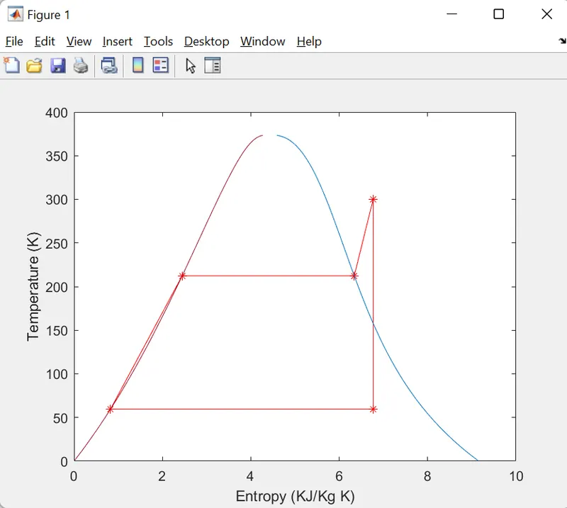
1)TS Diagram:-

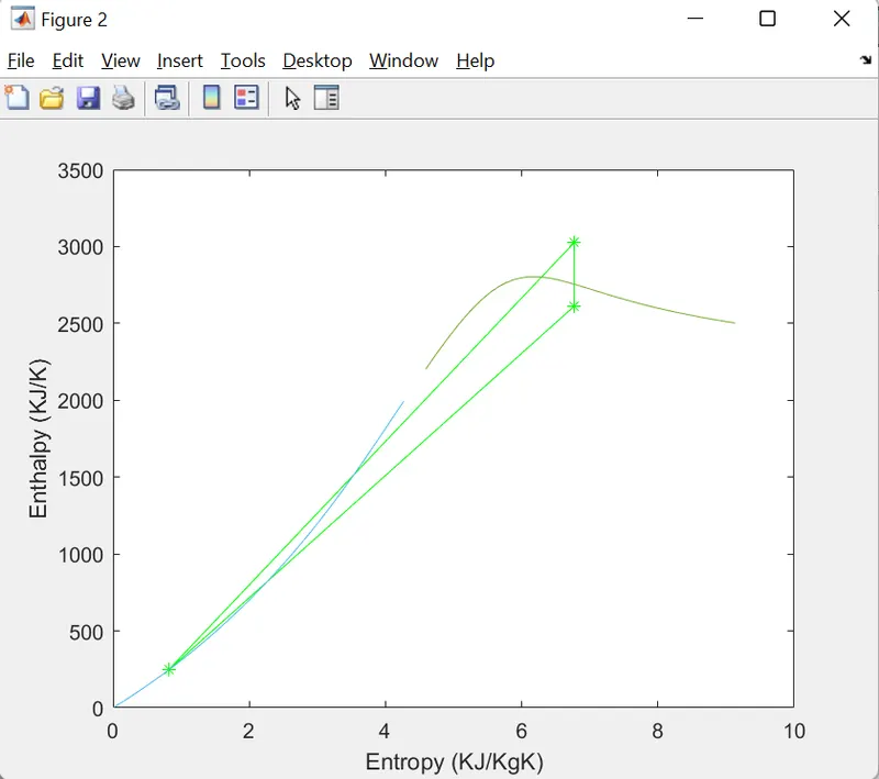
2) HS diagram:-

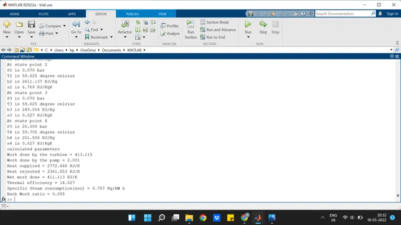
3) Calculated parameters:-

Errors Spotted:-

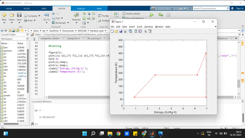
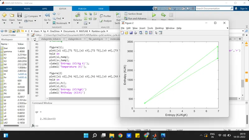
One of the major error I experienced was, the code for the 'for loop' had been mentioned as

'for i=length(temp)' instead of 'for i=1:length(temp)'.

So I didn't got the doom curve properly. The outpot was initially obtained as folllows:-

Reference:-

1) https://en.wikipedia.org/wiki/Rankine_cycle#:~:text=The%20Rankine%20cycle%20is%20an,heat%20source%20and%20heat%20sink.

2) https://byjus.com/jee-questions/what-are-the-four-processes-of-rankine-cycle/

3)https://skill-lync.com/student-projects/Project-2-Rankine-Cycle-Simulator-95692

Project 2 - Rankine cycle Simulator

Ship work like this
in your own course.

Talk to a career counsellor

Ship work like thisin your own course.

Talk to a career counsellor

Ship work like this
in your own course.