Challenge

Project 2 - Rankine cycle Simulator

SSibin Babu Mk1 May 2022

Aim

Create a Rankine Cycle Simulator using OCTAVE/MATLAB.
Code should calculate the state points of the Rankine Cycle based on user inputs (here Turbine Inlet temperature = 400° C, Turbine Inlet Pressure = 30 bars and Turbine Outlet Pressure = 0.05 bars = Condenser Inlet Pressure.)
Then, plot the corresponding T-s and h-s plots for the given set of inputs. Title and axes labels are a must, while legends could be used if necessary.
Use XSteam library to get steam table dataes.
Calculate back work ratio and net work done in rankine cycle

Methodology

Theory

Rankine Cycle

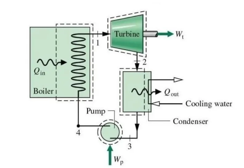
Rankine cycle is an idealiszed thermodynamic cycle that describes the production of mechanical work by the flow of fluid from the heat source to heat sink. Rankine cycle process widely used by power plants such as coal-fired power plants or nuclear reactors. In this mechanism, a fuel is used to produce heat within a boiler, converting water into steam which then expands through a turbine producing useful work. It consist of pump, boiler, turbine and condesor. The working fluid pumped into the boiler and heated using an external heat source and the steam produced expanded using a turbine which results in production of useful mechanical work. Expanded steam given to the condensor and the condensation takesplace which results in back to fluid state. The processes in rankine cycle are:

Process 1-2 : Isentropic expansion by Turbine - The working fluid(steam) from the boiler expands isentropicaly in turbine to produce usefull mechanical work (`W_t`). Here entropy is constant and pressure and temperature of the steam decreases.
Process 2-3 : Constant pressure heat rejection in condensor `Q_(out)`- Heat rejected out in condesor and condensation of steam takesplace at constant pressure to form saturated liquid.
Process 3-4 : Isentropic compression by the Pump - The saturated liquid from the condesor pumped to the boiler using a pump. Here it takeplace isentropicaly. Here work (`W_p`)is done on the pump.
Process 4-1 : Constant pressure heat addition in Boiler `Q_(add)` - The fluid pumped into the boiler heated using an external source and steam is produced which given to the turbine and cycle repeat. Enthalpy of liquid changes and pressure remains constant.

Saturated liquid : A liquid about to vapourise is called saturated liquid. If a small amount of heat added to saturated liquid it turns into vapour at constant temperature.

Saturated Vapour: A liquid about to condense is called saturated vapour. If a small amount of heat removed from saturated vapour it turns into liquid at constant temperature.

Governing Equations

Dryness Fraction = Mass of dry steam/ Mass of dry steam and mass of water vapour in the mixture
Work done by the Turbine (`W_t`) = `h_1-h_2`
Heat rejection by the condensor (`Q_(out)` = `h_2-h_3`
Work done by the pump (`W_p`) = `h_4-h_3`
Heat added to Boiler (Q_in) = `h_1-h_4`
Net work done W_net = `W_t-W_p`
Thermal Efficiency `T_(eff)` = Net work done / Heat addition = W_net/Q_in
Back work ratio BWR = (pump work input/turbine work output) = `W_p/W_t`

Notations Used

p1,p2,p3,p4 - Pressure at state points

t1,t2,t3,t4,t5,t6 - Temperature at state points

h1,h2,h3,h4,h5,h6 - Enthalpy at state points

s1,s2,s3,s4,s5,s6 - Entropy at state points

Sl2 - Saturated liquid entropy at state 2

Sv2 - Saturated vapour entropy at state 2

Hl2 - Saturated liquid enthalpy at state 2

Hv2 - Saturated vapour enthalpy at state 2

X - Dryness fraction

cp4 - Specific heat at constat pressure

cv4 -Specific heat at constant volume

Code

%Rankine cycle Simulator
%calculate the state points of the Rankine Cycle based on user input
clear all
close all
clc
% Headings
fprintf('               RANKINE CYCLE SIMULATOR             \n')

fprintf('Process(1-2) - Isentropic Expansion in the Turbine \n')
fprintf('Process(2-3) - Constant pressure heat rejection at condensor \n')
fprintf('Process(3-4) - Isentropic Compression in the pump \n')
fprintf('Process(4-1) - Constant pressure heat addition by the Boilor \n')

% User inputs
p1=input('Enter the Inlet pressure of turbine (in bar):');
p2=input('Enter the Inlet pressure of condensor (in bar):');
t1=input('Enter the Inlet temperature of turbine (in degree celcius):');

% Calculating Thermodynamic state conditions
% calculating state points-1 Turbine inlet (p1,t1,h1,s1)
h1=XSteam('h_pt',p1,t1); % h_pt - Enthalpy as a function of pressure and temperature
s1=XSteam('s_pt',p1,t1); % s_pt - Entropy as a function of pressure and temperature

% calculating state points-2 Condensor inlet (p2,t2,h2,s2)
% s1=s2 specific enthalpy is constant during isentropic process
s2=s1;
% calculating saturated liquid entropy state and vapour entropy state
Sl2=XSteam('sL_p',p2); % sL_p saturated liquid entropy
Sv2=XSteam('sV_p',p2); % sV_p saturated vapour entropy

% calculating saturated liquid enthalpy state and vapour enthalpy state
Hl2=XSteam('hL_p',p2); % hL_p saturated liquid enthalpy
Hv2=XSteam('hV_p',p2); % hV_p saturated vapour enthalpy
% calculating dryness fraction at state 2
X=(s2-Sl2)/(Sv2-Sl2);

% Enthalpy at poit 2
h2=Hl2+(X*(Hv2-Hl2));

% Calculating state variables at state -3 (p3,t3,h3,s3)
% pressure at point 2 and 3 are equal
p3=p2;
% Calculating saturation temperature
t3=XSteam('Tsat_p',p3);
t2=t3; % same temperature line
h3=XSteam('hl_p',p3); %saturated liquid enthalpy at p3
s3=XSteam('sl_p',p3); % saturated liquid entropy at p3

% Calculating state variables at state -4 (p4,t4,h4,s4)
s4=s3; %entropy same at state 3 and 4
p4=p1; %constant pressure heat addition 
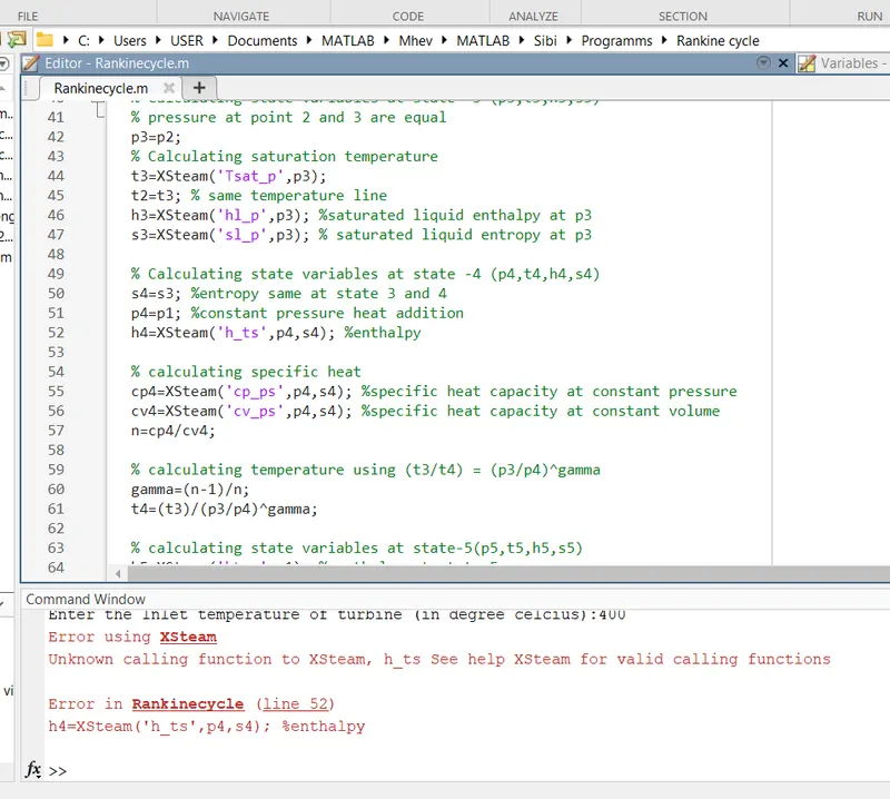
h4=XSteam('h_ps',p4,s4); %enthalpy

% calculating specific heat
cp4=XSteam('cp_ps',p4,s4); %specific heat capacity at constant pressure
cv4=XSteam('cv_ps',p4,s4) %specific heat capacity at constant volume
n=cp4/cv4;

% calculating temperature using (t3/t4) = (p3/p4)^gamma
gamma=(n-1)/n;
t4=(t3)/(p3/p4)^gamma;

% calculating state variables at state-5(p5,t5,h5,s5)
h5=XSteam('hL_p',p1); % enthalpy at state 5
s5=XSteam('sL_p',p1); % entropy at state 5

% calculating state variables at state-6(p6,t6,h6,s6)
s6=XSteam('sV_p',p1)
h6=XSteam('hV_p',p1);
t6=XSteam('Tsat_p',p1)
t5=t6;

% STATISTICAL ANALYSIS OF RANKAINE CYCLE
% work done by turbine
W_t=(h1-h2);

% work done by pump
W_p=(h4-h3);

% Net work done
W_net = W_t-W_p;

% Heat addition
Q_in = h1-h4;

% Heat Rejection
Q_out = h2-h3;

% Thermal efficiency = (network)/Heat addition
T_eff = (W_net/Q_in)*100;

% Back work ratio = pump work/turbine work
BWR = W_p/W_t;

% Specific steam consumption
SSC= 3600/W_net;

% Creating saturation curve using for loop
T=linspace(1,t1,1000);
for i=1:length(T)
    % liquid and vapour state enthalpy
    H_l(i)= XSteam('hL_t',T(i));
    H_v(i)=XSteam('hV_t',T(i));
    % Liquid and Vapour state entropy
    S_l(i)=XSteam('sL_t',T(i));
    S_v(i)=XSteam('sV_t',T(i));
end

% ploting T-S and H-S Diagram
% T-S diagram
figure(1)
hold on
text(s1,t1,'1')
plot([s1 s2], [t1 t2],'Color','r','LineWidth',1)
plot([s2 s3], [t2 t3],'Color','y','LineWidth',1)
text(s2,t2,'2')
plot([s3 s4], [t3 t4],'Color','b','LineWidth',1)
text(s3,t3,'3')
plot([s4 s5], [t4 t5],'Color','g','LineWidth',1)
text(s4,t4,'4')
plot([s5 s6], [t5 t6],'Color','c','LineWidth',1)
text(s5,t5,'5')
plot([s6 s1], [t6 t1],'Color','m','LineWidth',1)
text(s6,t6,'6')

%saturation curve 
plot(S_l,T,'LineStyle','-','color','b','LineWidth',1)
plot(S_v,T,'LineStyle','-','color','b','LineWidth',1)
xlabel('Entropy [Kj/Kg.k]')
ylabel('Temperature [Degree C]')
title('RANKAINE CYCLE T-S PLOT')
legend('Isentropic Expansion by Turbine','Constant pressure heat rejection in condensor','Isentropic compression by pump','Constant pressure Heat addition in liquid region','Heat addition during phase change','Heat addition during vapour region','Saturation curve')

% H-S diagram ploting
figure(2)
hold on
text(s1,h1,'1')
plot([s1 s2], [h1 h2],'Color','r','LineWidth',1)

plot([s2 s3], [h2 h3],'Color','g','LineWidth',1)
text(s2,h2,'2')
plot([s3 s4], [h3 h4],'Color','b','LineWidth',1)
text(s3,h3,'3')
plot([s4 s1], [h4 h1],'Color','y','LineWidth',1)
text(s4,h4,'4')

% Saturation curve
plot(S_l,H_l,'LineStyle','-','color','b','LineWidth',1)
plot(S_v,H_v,'LineStyle','-','color','b','LineWidth',1)
xlabel('Entropy [Kj/Kg.k]')
ylabel('Enthalpy [Kj/Kg]')
title('RANKAINE CYCLE H-S PLOT')
legend('Isentropic Expansion by Turbine','Constant pressure heat rejection in condensor','Isentropic compression by pump','Constant pressure Heat addition in Boiler','Saturation curve')

fprintf('               Thermodynamic State points                  \n')
fprintf('At state 1: \n')
fprintf('P1=%.3f bar \n', p1)
fprintf('T1=%.3f degree celcius \n', t1)
fprintf('H1=%.3f Kj/Kg \n', h1)
fprintf('S1=%.3f Kj/Kg-K \n', s1)

fprintf('At state 2: \n')
fprintf('P2=%.3f bar \n', p2)
fprintf('T2=%.3f degree celcius \n', t2)
fprintf('H2=%.3f Kj/Kg \n', h2)
fprintf('S2=%.3f Kj/Kg-K \n', s2)

fprintf('At state 3: \n')
fprintf('P3=%.3f bar \n', p3)
fprintf('T3=%.3f degree celcius \n', t3)
fprintf('H3=%.3f Kj/Kg \n', h3)
fprintf('S3=%.3f Kj/Kg-K \n', s3)

fprintf('At state 4: \n')
fprintf('P4=%.3f bar \n', p4)
fprintf('T4=%.3f degree celcius \n', t4)
fprintf('H4=%.3f Kj/Kg \n', h4)
fprintf('S4=%.3f Kj/Kg-K \n', s4)

fprintf('               Statistical Result Of Rankine Cycle                \n ')
fprintf('work done by turbine W_t=%.3f Kj/Kg \n',W_t)

fprintf('work done by pump W_p=%.3f Kj/Kg \n',W_p)

fprintf('Net work done W_net=%.3f Kj/Kg \n',W_net)

fprintf('Heat addition Q_in=%.3f Kj \n',Q_in)

fprintf('Heat Rejection Q_out=%.3f Kj \n',Q_out)

fprintf('Thermal efficiency T_eff = %.3f  \n',T_eff)

fprintf('Back work ratio BWR=%.3f \n',BWR)

fprintf('Specific steam consumption SSC= %.3f \n',SSC)

Code Explanation

Using fprintf command the processes of rankaine cycle is displayed.
using input command the inlet pressure of turbine, inlet pressure of condensor and inlet temperature of turbine are read as user inputs.
using XSteam function read the steam table data of water and water vapour are read and using it calculate the enthlpy and entropy at state points.

h1=XSteam('h_pt',p1,t1); h_pt - Enthalpy as a function of pressure and temperature enthlpy at state poit 1 calculated.

s1=XSteam('s_pt',p1,t1); s_pt - Entropy as a function of pressure and temperature entropy is calculated.
calculate state points-2 Condensor inlet (p2,t2,h2,s2)

s1=s2 specific enthalpy is constant during isentropic process. calculate saturated liquid entropy state and vapour entropy state using XSteam function.

Sl2=XSteam('sL_p',p2); sL_p saturated liquid entropy

Sv2=XSteam('sV_p',p2); sV_p saturated vapour entropy and also calculate saturated liquid enthalpy state and vapour enthalpy state Hl2=XSteam('hL_p',p2); hL_p saturated liquid enthalpy Hv2=XSteam('hV_p',p2); hV_p saturated vapour enthalpy also calculating dryness fraction at state 2 using

X=(s2-Sl2)/(Sv2-Sl2); X-dryness fraction.

Enthalpy at poit 2 is calculated using the equation h2=Hl2+(X*(Hv2-Hl2)).
Calculate state variables at state -3 (p3,t3,h3,s3) here pressure at point 2 and 3 are equal

p3=p2; Calculate saturation temperature using XSteam function.

t3=XSteam('Tsat_p',p3);

t2=t3; same temperature line

h3=XSteam('hl_p',p3); saturated liquid enthalpy at p3

s3=XSteam('sl_p',p3); saturated liquid entropy at p3
Calculate state variables at state -4 (p4,t4,h4,s4)

s4=s3; entropy same at state 3 and 4

p4=p1; constant pressure heat addition

h4=XSteam('h_ps',p4,s4); enthalpy at state 4
calculate specific heat

cp4=XSteam('cp_ps',p4,s4); specific heat capacity at constant pressure

cv4=XSteam('cv_ps',p4,s4) specific heat capacity at constant volume

n=cp4/cv4;

Calculate the temperature using (t3/t4) = (p3/p4)^gamma where gamma=(n-1)/n;

t4=(t3)/(p3/p4)^gamma;
Using same method and XSteam function calculate the state points at state 5 and 6.
Calculate the various parameters associated with rankine cycle by using the equations given below

work done by turbine

W_t=(h1-h2);

work done by pump

W_p=(h4-h3);

Net work done

W_net = W_t-W_p;

Heat addition

Q_in = h1-h4;

Heat Rejection

Q_out = h2-h3;

Thermal efficiency = (network)/Heat addition

T_eff = (W_net/Q_in)*100;

Back work ratio = pump work/turbine work

BWR = W_p/W_t;

Specific steam consumption

SSC= 3600/W_net;
Produce the values for satuaration curve, that is liquid and vapour state enthalpy and entropy using a for loop. Temperature array for the 'For' loop is produced by using the linspace command T=linspace(1,t1,1000) which produces 1000 temperature points in between 1 and temperature t1.
Draw the saturation curve for T-S diagram using plot command

plot(S_l,T,'LineStyle','-','color','b','LineWidth',1)

plot(S_v,T,'LineStyle','-','color','b','LineWidth',1)

For H-S diagram using

plot(S_l,H_l,'LineStyle','-','color','b','LineWidth',1)

plot(S_v,H_v,'LineStyle','-','color','b','LineWidth',1)
Plot the Temperature -Entropy diagram and Enthalpy-Entropy diagram using plot command.
plot([s1 s2], [t1 t2],'Color','r','LineWidth',1) T-S diagram process 1 to 2
plot([s1 s2], [h1 h2],'Color','r','LineWidth',1) H-S diagram process 1-2.

Proper labeling is provided using xlabel and ylabel and legend is provided using legend command.
Thermodynamic state points and the various parameters are displayed on the screen using fprintf command.

Output

T-S Plot

H-S Plot

Command Window

Errors encountered

Error occured due to improper defining of XSteam function. Corrected by properly defining it.

Conclusion

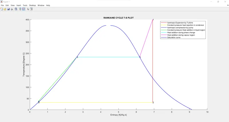
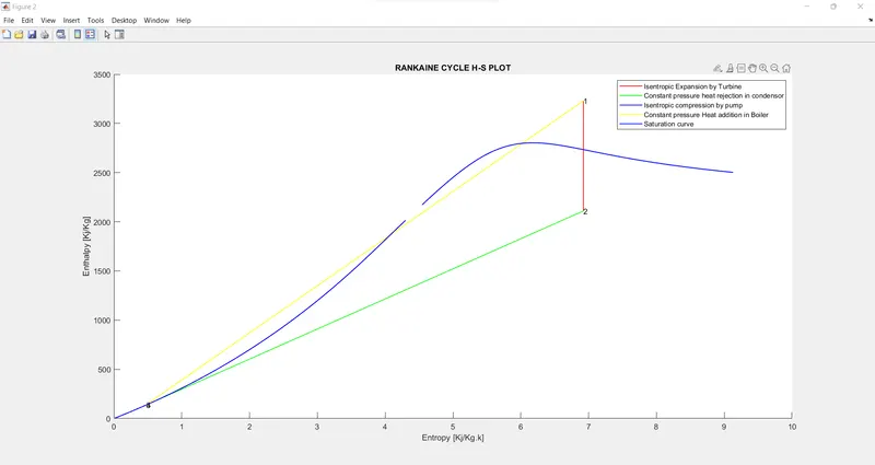
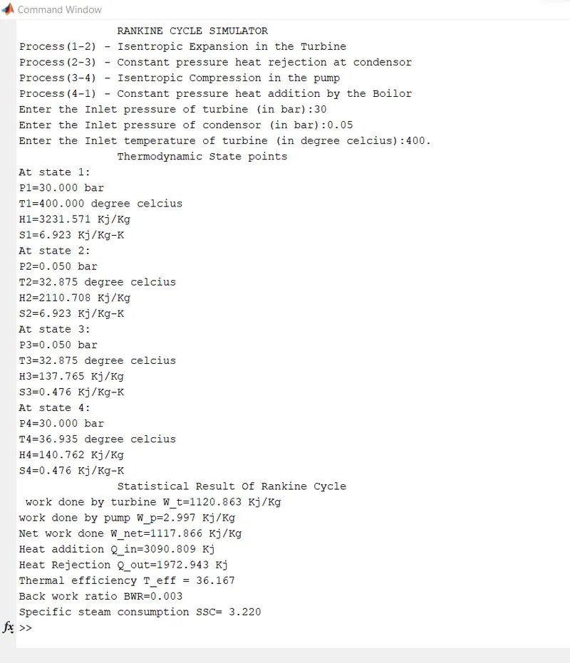
The code to simulate the Rankaine cycle is done successfully using matlab.
calculated the state points of the Rankine Cycle based on user inputs (here Turbine Inlet temperature = 400° C, Turbine Inlet Pressure = 30 bars and Turbine Outlet Pressure = 0.05 bars = Condenser Inlet Pressure) and diyplayed properly.
Plot the T-S and H-S graph for rankine cycle.
Calculated Back work ratio BWR= 0.003 and Net work output = 1117.866 Kj/Kg.

References

Project 2 - Rankine cycle Simulator

Ship work like this
in your own course.

Talk to a career counsellor

Ship work like thisin your own course.

Talk to a career counsellor

Ship work like this
in your own course.