Project 2 - Rankine cycle Simulator

AIM: To create a Rankine Cycle Simulator form given input and reading the data from stadard thermodynamic library of steam table.

OBJECTIVE:

1. To create a Rankine Cycle simulator in MATLAB.
2. To calculate the state point using function XSteam. Work Done and Efficiency of the Rankine Cycle.
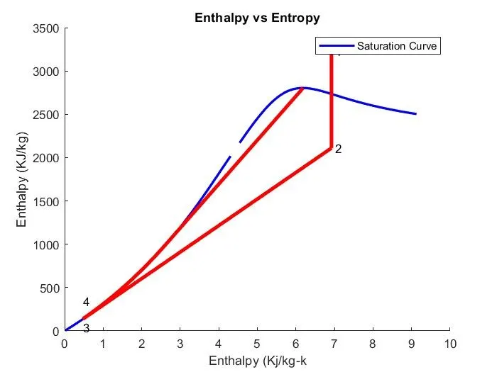
3. To plot T-S & H-S curve for given inut in Rankine Cycle.
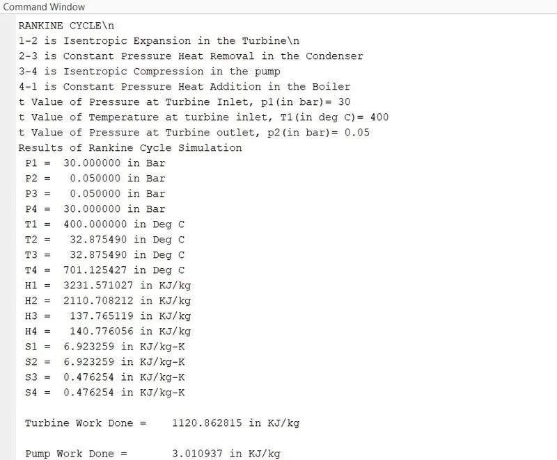
4. To get output in the command window for each state point of cycle.

THEORY:

The Rankine Cycle is an idealized thermodynamic cycle describing the process by which certain heat engines, such as steam turbines or reciprocating steam engines, allow mechanical work to be extracted from a fluid as it moves between a heat source and heat sink.

Possible heat sources include combustion of fossil fuels (such as coal, natural gas or oil) or renewable fuels (like biomass or ethanol, nuclear fission and concentrated solar power). Common heat sinks include ambient air above or around a facility and bodies of water ( like rivers, ponds and oceans).

The ability of Rankine engine to harness energy depends on the relative tempertaure difference between the heat source and heat sink. The greater the differential, the more mechanical power can be efficiently extracted out of heat energy, as per Carnot's theory.

The efficiency of the Rankine Cycle is limited by the high heat of vaporization of the working fluid. Rankine engines generally operate in a closed loop where the working fluid is reused. Water is usually chosen as the working fluid for its simple chemistry, relative abundance, low cost, non toxic and thermodynamic properties.

fig: physical layout of the Rankine Cycle

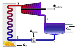
where, 1.Pump, 2.Boiler, 3.Turbine and 4.Condenser

PROCESSES & WORKING in RANKINE CYCLE:

There are 4 processes in the Rankine cycle:

1. Process 1-2 (Isentropic compression): The working fluid is pumped from low to high pressure. The fluid is in its liquid state, thus a little input enery is requied by the pump.
2. Process 2-3 (Constant Pressure heat addition in boiler): The high pressure fluid enters a boiler, where it is heated at constant pressure by a external heat source to be come a dry saturated vapour.
3. Process 3-4 (Isentropic Expansion): The dry saturated vapour through a trubinem generating power. This decreases the temperature and pressure of the vapour, and some condensation may occur.
4. Process 4-1 (Constant Pressure heat rejection in condenser): The wet vapour then enters a condenser, where it is condensed at a constant pressure to become a saturated liquid.

We are considering an ideal Rankine cycle as it differs from the actual vapour power cycle because of the irreversibilities in the inherent components caused by fluid friction and heat loss to the surroundings; fluid friction causes pressure drops in the boiler, the condenser, and the piping between the components, and as a result the steam leaves the boiler at a lower pressure; heat loss reduces the net work output, thus heat addition to the steam in the boiler is required to maintain the same level of net work output.

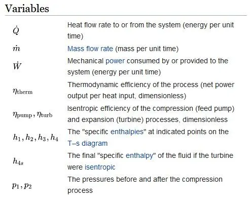
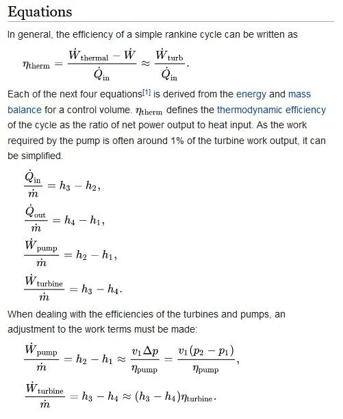
Net Work done: W(net) = Q(in) - Q(out) = W(turbine) - W(pump)

CODE:

%% Rankine Cycle Simulator

clear all
close all
clc

%% Displaying info
disp('RANKINE CYCLE\n');
disp('1-2 is Isentropic Expansion in the Turbine\n');
disp('2-3 is Constant Pressure Heat Removal in the Condenser');
disp('3-4 is Isentropic Compression in the pump');
disp('4-1 is Constant Pressure Heat Addition in the Boiler');

%% Obtaining Input Data
p1 = input('\t Value of Pressure at Turbine Inlet, p1(in bar)= ');
T1 = input('\t Value of Temperature at turbine inlet, T1(in deg C)= ');
p2 = input('\t Value of Pressure at Turbine outlet, p2(in bar)= ');

%% Extracting data 
% State 1
h1 = XSteam('h_pT', p1, T1); %extracting enthalpy at state point 1
s1 = XSteam('s_pT', p1, T1); %extracting entropy at state point 1

% State 2
s2 = s1; % Isentropic Expansion
sf2 = XSteam('sL_p', p2); % Saturated liquid Entropy
sg2 = XSteam('sV_p', p2); % Saturated vapour Entropy
x2 = (s2-sf2)/(sg2-sf2);
hf2 = XSteam('hL_p',p2);
hg2 = XSteam('hV_p', p2);
h2 = hf2 + (x2*(hg2-hf2));

% State 3
p3 = p2; % constant pressure heat rejection in condenser
s3 = XSteam('sL_p', p3);
h3 = XSteam('hL_p', p3);

% State 4
s4 = s3; % Isentropic compression
p4 = p1;  %pressure output at point 4 = pressure input at point 1

% Work Done by turbine
Wt = h1 - h2;

% Work Done by pump
v3 = XSteam('vL_p', p3);
Wp = v3*(p4-p3)*100;
h4 = h3 + Wp;

% Net Work
Wnet = Wt - Wp;

% Heat into system
Qin = h1 - h4;

% Heat out of system
Qout = h2 - h3;

% Thermal Efficiency
Teff = (Wnet/Qin)*100;

% Specific Steam Consumption ( SSC = mass flow rate/power)
SSC = (3600/Wnet);

% Calculation of data at state points
T3 = XSteam('Tsat_p', p3);
T2 = T3;
Cp4 = XSteam('Cp_ps', p4, s4);
Cv4 = XSteam('Cv_ps', p4, s4);
k = Cp4/Cv4;
T4 = T3/((p3/p4^((k-1)*k)));

% Calculation of data at the vapour and liquid conditions of fluid
T6 = XSteam('Tsat_p',p1);
s5 = XSteam('sL_p', p1);
s6 = XSteam('sV_p', p1);
h5 = XSteam('hL_p', p1);
h6 = XSteam('hV_p', p1);
T5 = T6;

% PLotting for saturation Line
T = linspace(1,560,1000);
for i = 1:length(T)
    sf(i) = XSteam('sL_T',T(i)); % Saturated liquid Entropy
    sg(i) = XSteam('sV_T', T(i)); % Saturated Vapour Entropy
    hf(i) = XSteam('hL_T',T(i)); % Saturated Liquid Enthalpy
    hg(i) = XSteam('hV_T', T(i)); % Saturated Vapour Enthalpy
end

% Plotting T-S Diagram for Rankine Cycle
figure(1)
hold on
plot(sf, T, 'color','b','linewidth',2)
plot(sg,T,'color','b','linewidth',2)
plot([s1 s2],[T1 T2], 'color', 'r', 'LineWidth',3)
plot([s2 s3],[T2 T3], 'color', 'r', 'LineWidth',3)
plot([s3 s4],[T3 T4], 'color', 'r', 'LineWidth',3)
plot([s4 s5],[T4 T5], 'color', 'r', 'LineWidth',3)
plot([s5 s6],[T5 T6], 'color', 'r', 'LineWidth',3)
s_1 = linspace(s6,s1,1000);
for j = 1:length(s_1)
    Tc(j) = XSteam('T_ps',p1,s_1(j));
end
plot(s_1,Tc,'color','r','LineWidth',3)
text(s1+0.1, T1,'1')
text(s2+0.1,T2,'2')
text(s3,T3-20,'3')
text(s4,T4+20,'4')
title('Temperature vs Entropy')
xlabel('Entropy (Kj/kg-k)')
ylabel('Temperature (Deg C)')
legend('Saturation Curve')

% PLotting H-S Diagram for Rankine Cycle
figure(2)
hold on
plot(sf,hf,'color','b','LineWidth',2)
plot(sg,hg,'color','b','LineWidth',2)
plot([s1 s2], [h1 h2],'color','r','LineWidth',3)
plot([s2 s3], [h2 h3],'color','r','LineWidth',3)
plot([s3 s4], [h3 h4],'color','r','LineWidth',3)
hc = linspace(h4,h5,100);
for k = 1:length(hc)
    s_c(k) = XSteam('s_ph',p1,hc(k));
end
plot(s_c,hc,'color','r','LineWidth',3)
plot([s5 s6],[h5 h6],'color','r','LineWidth',3)
for l = 1:length(s_1)
    h_c(1) = XSteam('h_ps',p1,s_1(1));
end
plot(s_1,h_c,'color','r','LineWidth',3)
text(s1+0.1,h1,'1')
text(s2+0.1,h2,'2')
text(s3,h3-100,'3')
text(s4,h4+200,'4')
title('Enthalpy vs Entropy')
xlabel('Enthalpy (Kj/kg-k')
ylabel('Enthalpy (KJ/kg)')
legend('Saturation Curve')

%% Displaying Results 

disp('Results of Rankine Cycle Simulation')
fprintf(' P1 = %10f in Bar\n',p1);
fprintf(' P2 = %10f in Bar\n',p2);
fprintf(' P3 = %10f in Bar\n',p3);
fprintf(' P4 = %10f in Bar\n',p4);
fprintf(' T1 = %11f in Deg C\n',T1);
fprintf(' T2 = %11f in Deg C\n',T2);
fprintf(' T3 = %11f in Deg C\n',T3);
fprintf(' T4 = %11f in Deg C\n',T4);
fprintf(' H1 = %12f in KJ/kg\n',h1);
fprintf(' H2 = %12f in KJ/kg\n',h2);
fprintf(' H3 = %12f in KJ/kg\n',h3);
fprintf(' H4 = %12f in KJ/kg\n',h4);
fprintf(' S1 = %9f in KJ/kg-K\n',s1);
fprintf(' S2 = %9f in KJ/kg-K\n',s2);
fprintf(' S3 = %9f in KJ/kg-K\n',s3);
fprintf(' S4 = %9f in KJ/kg-K\n',s4);
fprintf('\n Turbine Work Done = %14f in KJ/kg\n',Wt);
fprintf('\n Pump Work Done = %14f in KJ/kg\n',Wp);
fprintf('\n Wnet = %14f KJ/kg\n',Wnet);
fprintf('\n Efficiency = %14f % \n',Teff);
fprintf('S.S.C = %10f KJ/KWh\n',SSC);

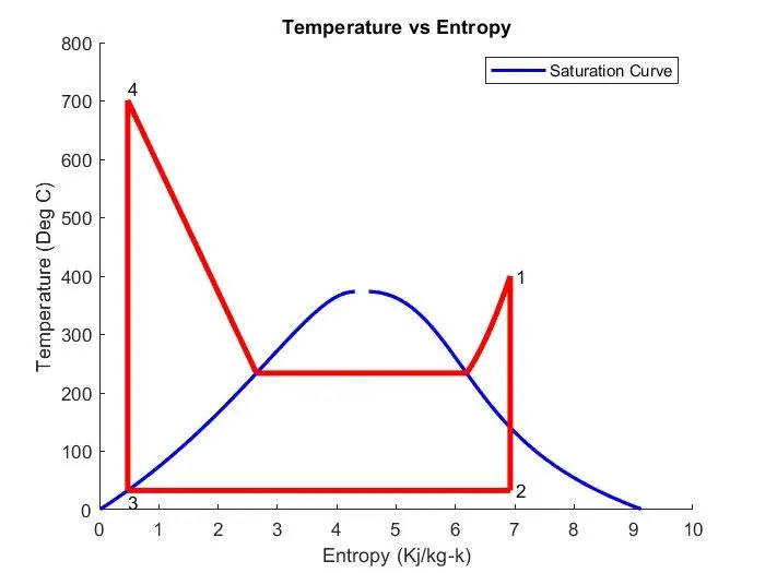
PLOTS:

[T vs S]:

[H vs S]:

Command Window Results:

###################################################

RANKINE CYCLE\n
1-2 is Isentropic Expansion in the Turbine\n
2-3 is Constant Pressure Heat Removal in the Condenser
3-4 is Isentropic Compression in the pump
4-1 is Constant Pressure Heat Addition in the Boiler
t Value of Pressure at Turbine Inlet, p1(in bar)= 30
t Value of Temperature at turbine inlet, T1(in deg C)= 400
t Value of Pressure at Turbine outlet, p2(in bar)= 0.05
Results of Rankine Cycle Simulation
P1 = 30.000000 in Bar
P2 = 0.050000 in Bar
P3 = 0.050000 in Bar
P4 = 30.000000 in Bar
T1 = 400.000000 in Deg C
T2 = 32.875490 in Deg C
T3 = 32.875490 in Deg C
T4 = 701.125427 in Deg C
H1 = 3231.571027 in KJ/kg
H2 = 2110.708212 in KJ/kg
H3 = 137.765119 in KJ/kg
H4 = 140.776056 in KJ/kg
S1 = 6.923259 in KJ/kg-K
S2 = 6.923259 in KJ/kg-K
S3 = 0.476254 in KJ/kg-K
S4 = 0.476254 in KJ/kg-K

Turbine Work Done = 1120.862815 in KJ/kg

Pump Work Done = 3.010937 in KJ/kg

Wnet = 1117.851878 KJ/kg

Efficiency = 36.167131 S.S.C = 3.220462 KJ/KWh
####################################################

EXPLANATION:

• XSteam data file is used to extract steam and water properties of enthalpy, entropy at specific pressure and temperatures for saturated liquid, saturated vapour condinations etc.
• The programs asks for the Input pressure at point 1 (in Bar), Input Temperature at same point (in deg C), and Pressure at point 2 (in Bar).
• As per the question P1 = 30 bar, T1 = 400 deg C, and P2 = 0.05 bar.
• With the help of the inputs, and the XSteam data file, we extract the data of the enthalpy, entropy at each state of the Rankine Cycle.
• sf, sg, hf, hg are the entropy and enthalpy of saturated liquid(f) and saturated vapour(g).
• The net work, Work done by pump and turbine, Heat in and out are calculated using the standard thermodynamic relations.
• Efficiency and Specific Steam Consumption(S.S.C) of the RAnkine Cycle is claculated.
• Respective plots as shown above are obtained from the program.
• The plot changes with the change of input values provided by the user.
• The results are displayed in the command window.

REFERENCES:

• https://en.wikipedia.org/wiki/Rankine_cycle