Challenge

Rankine cycle Simulator using MATLAB.

VVivek Nair23 Sept 2022

AIM: Create a Rankine Cycle Simulator using MATLAB.

OBJECTIVE:

Calculate the state points of the Rankine Cycle based on user inputs.
Plot the corresponding T-s and h-s plots for the given set of inputs.
Calculate Net work output and Back work ratio.

THEORY:

ldeal Rankine Cycle:

The Rankine cycle system consists of a pump, boiler, turbine, and condenser. The pump delivers liquid water to the boiler. The boiler heated water with the help of the furnace converts water to superheated steam. This steam is used to run the turbine which powers the generator. Steam leaves the turbine and becomes cooled to a liquid state in the condenser. Then the liquid is pressurized by the pump and goes back to the boiler. And the cycle continues. The figure is as follow,

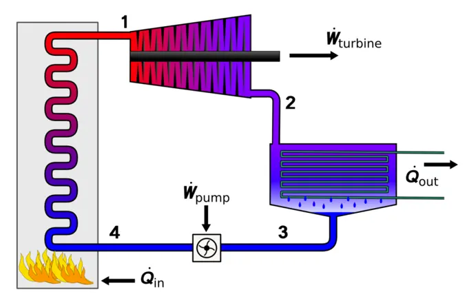
In an ideal Rankine cycle, all the units operate with the steady-state flow, and the kinetic and potential energy of the fluid is considered to be negligible compared to the temperature and pressure effects. The Rankine cycle efficiency is much higher than Carnot cycle efficiency because the pump is used in the Rankine cycle, which gives a higher work ratio by doing a significant proportion of turbine work.

Working Principle:

There are four processes in the Rankine cycle. The states are identified by numbers (in brown) in the T-S diagram.

Process 1–2, Isentropic or Reversible Adiabatic Expansion (Turbine): The working fluid is pumped from low to high pressure. As the fluid is a liquid at this stage, the pump requires little input energy. Process 1-2 is isentropic compression.
Process 2–3, Constant Pressure Heat Rejection (Condenser): The high-pressure liquid enters a boiler, where it is heated at constant pressure by an external heat source to become a dry saturated vapour. The input energy required can be easily calculated graphically, using an enthalpy - entropy chart (h-s chart, or Mollier diagram), or numerically, using steam tables or software. Process 2-3 is constant pressure heat addition in the boiler.
Process 3–4, Isentropic or Reversible Adiabatic Compression (Pump): The dry saturated vapour expands through a turbine, generating power. This decreases the temperature and pressure of the vapour, and some condensation may occur. The output in this process can be easily calculated using the chart or tables noted above. Process 3-4 is isentropic expansion.
Process 4–1, Constant Pressure Heat Addition (Boiler): The wet vapour then enters a condenser, where it is condensed at a constant pressure to become a saturated liquid. Process 4-1 is constant pressure heat rejection in the condenser.

In an ideal Rankine cycle, the pump and turbine would be isentropic, i.e., the pump and turbine would generate no entropy and hence maximize the net work output. Processes 1–2 and 3–4 would be represented by vertical lines on the T-S diagram and more closely resemble that of the Carnot cycle. The Rankine cycle shown here prevents the state of the working fluid from ending up in the superheated vapor region after the expansion in the turbine, which reduces the energy removed by the condensers.

The actual vapor power cycle differs from the ideal Rankine cycle because of irreversibilities in the inherent components caused by fluid friction and heat loss to the surroundings; fluid friction causes pressure drops in the boiler, the condenser, and the piping between the components, and as a result, the steam leaves the boiler at a lower pressure; heat loss reduces the net work output, thus heat addition to the steam in the boiler is required to maintain the same level of net work output.

PROCEDURE:

The command for the Rankine Cycle Simulator:

clear all
close all
clc

% Rankine Cycle Process
disp('      RANKINE CYCLE SIMULATOR')
fprintf('n')
disp('1-2 Isentropic Expansion in Turbine')
disp('2-3 Constant Pressure Heat Rejection in Condenser')
disp('3-4 Isentropic Compression in Pump')
disp('4-1 Constant Pressure Heat Addition in Boiler')
fprintf('n')

% Obtaining the input Data.
p1 = input('Turbine inlet Pressure in (bar), p1 = ');
t1 = input('Turbine inlet Temperature in (degree celcius), t1 = ');
p2 = input('Condenser inlet Pressure in (bar), p2 = ');
fprintf('n')

% State 1 Boiler Outlet or Turbine Inlet
% Enthalpy at Point 1
s1 = XSteam('s_pT',p1,t1);
h1 = XSteam('h_pT',p1,t1);

% State 2 Turbine Outlet or Condenser Inlet
% Constant Pressure Heat Rejection in Condenser
s2 = s1;
t2 = XSteam('Tsat_p',p2);
% Saturated Liquid Entropy
sf2 = XSteam('sl_p',p2);
% Saturated Vapour Entropy
sg2 = XSteam('sV_p',p2);
% Saturated Liquid Enthalpy
hf2 = XSteam('hL_p',p2);
% Saturated Vapour Enthalpy 
hg2 = XSteam('hV_p',p2);
% Vapour Fraction
x2 = ((s2-sf2)/(sg2-sf2));
% Enthalpy at Point 2
h2 = hf2+(x2*(hg2-hf2));

% State 3 Condenser Outlet or Pump Inlet
p3 = p2;
t3 = t2;
s3 = XSteam('sL_p',p3);
h3 = XSteam('hL_p',p3);
v3 = XSteam('vL_p',p3);

% State 4 Pump Outlet or Boiler Inlet
% Constant Pressure Heat Addition in Boiler
p4 = p1;
s4 = s3;
cp4 = XSteam('Cp_ps',p4,s4);
cv4 = XSteam('Cv_ps',p4,s4);
g4 = cp4/cv4;
o = (g4-1)/g4;
t4 = t3*((p4/p3)^o);

% Work done by Pump
Wp = v3*(p4-p3)*100;

h4 = h3+Wp;

% State 5
s5 = XSteam('sL_p',p1);
h5 = XSteam('hL_p',p1);
t5 = XSteam('Tsat_p',p1);

% State 6
s6 = XSteam('sV_p',p1);
h6 = XSteam('hV_p',p1);
t6 = t5;

% Work done by Turbine
Wt = h1-h2;

% Net Work done
Wnet = Wt-Wp;

% Heat in
Qin = h1-h4;

% Heat out
Qout = h2-h3;

% Thermal Efficiency
eff = Wnet/Qin;

% Creating an Array for Temperature
T = linspace(0,400,1000);

% Entropy and Enthalpy values for creating Saturation Curve
for i=1:length(T)
    sf(i)=XSteam('sL_T',T(i));
    sg(i)=XSteam('sV_T',T(i));
    hf(i)=XSteam('hL_T',T(i));
    hg(i)=XSteam('hV_T',T(i));
end

% Plotting T-S Diagram for Cycle
figure(1)
plot(sf,T,'linewidth',1.5)
hold on
plot(sg,T,'linewidth',1.5)
plot([s1,s2],[t1,t2],'linewidth',1.5,'color','k')
plot([s2,s3],[t2,t3],'linewidth',1.5,'color','k')
plot([s3,s4],[t3,t4],'linewidth',1.5,'color','k')
plot([s4,s5],[t4,t5],'linewidth',1.5,'color','k')
plot([s5,s6],[t5,t6],'linewidth',1.5,'color','k')
plot([s6,s1],[t6,t1],'linewidth',1.5,'color','k')
legend('Saturated Liquid','Saturated Vapour')
axis([0 8 0 450])
grid on 
xlabel('Entropy(S)')
ylabel('Temperature(T)')
title('Temperature(T) V/S Entropy(S)')
saveas(figure(1),'T vs S.jpg')

% Plotting H-S Diagram for Cycle
figure(2)
plot(sf,hf,'linewidth',1.5,'color','r')
hold on
plot(sg,hg,'linewidth',1.5,'color','r')
plot([s1,s2],[h1,h2],'linewidth',1.5,'color','k')
plot([s2,s3],[h2,h3],'linewidth',1.5,'color','k')
plot([s3,s4],[h3, h4],'linewidth',1.5,'color','k')
plot([s4,s5],[h4,h5],'linewidth',1.5,'color','k')
plot([s5,s6],[h5,h6],'linewidth',1.5,'color','k')
plot([s6,s1],[h6,h1],'linewidth',1.5,'color','k')
grid on
legend('Saturation curve')
axis([0 8 0 450])
xlabel('Entropy(S)')
ylabel('Entahlpy(H)')
title('Enthalpy(H) VS Entropy(S)')
saveas(figure(2),'H vs S.jpg')

% Back work ratio
Back_work_ratio = (h4-h3)/(h1-h2);

% SSC
SSC = 3600/(h1-h2);

% Displaying Results
disp('      RESULTS')
fprintf('n')
fprintf('State point 1:n')
fprintf('P1 = %f bar n',p1)
fprintf('T1 = %f *Cn',t1)
fprintf('H1 = %f KJ/Kgmn',h1)
fprintf('S1 = %f KJ/Kg-kn',s1)
fprintf('n')

fprintf('state point 2:n')
fprintf('P2 = %f bar n',p2)
fprintf('T2 = %f *Cn',t2)
fprintf('H2 = %f KJ/Kgmn',h2)
fprintf('S2 = %f KJ/Kg-kn',s2)
fprintf('X2 = %f n',x2)
fprintf('n')

fprintf('State point 3:n')
fprintf('P3 = %f bar n',p3)
fprintf('T3 = %f *Cn',t3)
fprintf('H3 = %f KJ/Kgmn',h3)
fprintf('S3 = %f KJ/Kg-kn',s3)
fprintf('n')

fprintf('State point 4:n')
fprintf('P4 = %f bar n',p4)
fprintf('T4 = %f *Cn',t4)
fprintf('H4 = %f KJ/Kgmn',h4)
fprintf('S4 = %f KJ/Kg-kn',s4)
fprintf('n')

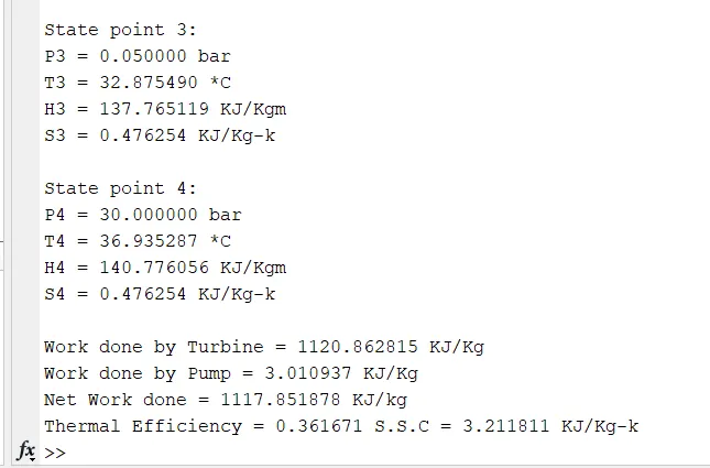
fprintf('Work done by Turbine = %f KJ/Kgn',Wt)
fprintf('Work done by Pump = %f KJ/Kgn',Wp)
fprintf('Net Work done = %f KJ/kgn',Wnet)
fprintf('Thermal Efficiency = %f %n',eff)
fprintf('S.S.C = %f KJ/Kg-kn',SSC)

Explanation of the Program:

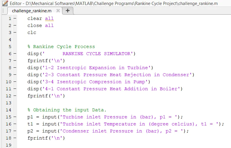
clear all - To clear all variables from the current workspace.
close all - close all figures whose handles are visible.
clc - clears all the text from the Command Window.
disp - The disp command is used to display the written text in the brackets in the command window.
fprintf - The fprintf command displays formatted text centered on the icon and can display formatSpec along with the contents of var.
fprintf('n') - This command is used to skip a line so that the command window is more presentable.
Line 6 to 12 - The disp command is used to display the heading of the program and the process that is included in the Rankine Cycle.
Line 15 to 18 - Defining the user-defined inputs. (p1,t1,p2).
input - This command is used to input some specific value to the problem solving, in this program is it assigned to inputs values of (p1,t1,t2) in the command window to solve the Rankine Cycle.
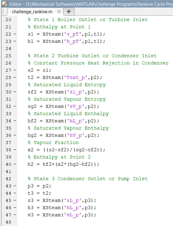
Line 20 to 23 - Extracting values of entropy and enthalpy from the XSteam function file for State 1.
Line 25 to 40 - Extarting values of entropy, temperature, saturated liquid entropy, saturated vapour entropy, saturated liquid enthalpy, saturated vapour enthalpy, vapour fraction, and the enthalpy from the Xsteam function file for State 2.
Line 42 to 47 - I defined the values of pressure and temperature for state 3, and extracted the values for entropy, enthalpy, and volume for state 3.
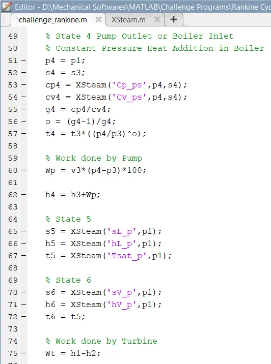
Line 49 to 57 - Writing down the equation for the values of pressure, entropy, and temperature at state 4. Then extracting the values for Specific isobaric heat capacity and Specific isochoric heat capacity for state 4 so that I can use these values for the calculation good the g and o values also.
Line 59 to 62 - Writing down the formula for the calculation of the Work done by the Pump.
Line 59 to 75 - Extracting values of entropy, enthalpy, and temperature from the XSteam function file for states 5&6. Writing down the formula for the work done by the turbine.
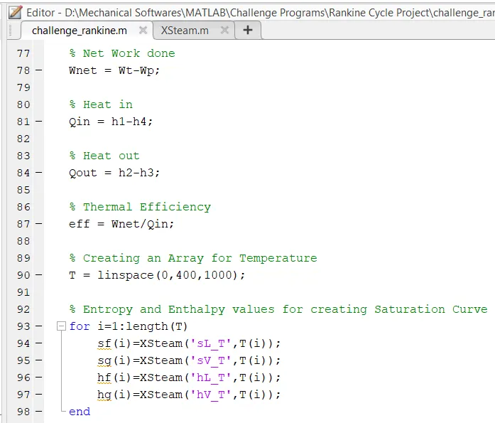
Line 77 to 90 - Writing down the formulas for the calculation of Net Work done, Heat in, Heat out, Thermal Efficiency. I also created an array using the linspace command for the Temperature.
linspace - The linspace function generates linearly spaced vectors.
Line 92 to 98 - Creating a for loop for the calculation of sf, sg, hf, and hg using the XSteam function file. Using the end command to stop the for loop.
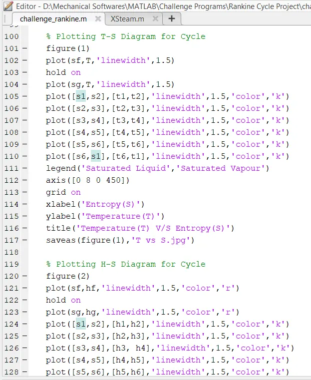
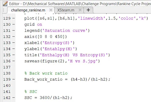
figure - The figure command is given so that the plots will be two different ones.
linewidth - The line width command is given to give width to the line which is gonna be plotted on the graph.
hold on - It is used so that there will be a pause in the plotting.
Line 100 to 136 - Plotting commands for the Plotting of T-s and H-S diagram.
legend - It is used for the indication of the line.
axis - For assigning axis for the plot.
xlabel - For the labeling of the x-axis.
ylabel - For the labeling of the y-axis.
title - For giving title to the graphs.
saveas - To save the plot file to the directory.
Line 139 - Writing the formula for back work ratio.
Line 142 - Writing the formula for SSC.
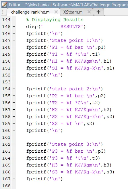
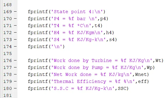
Line 144 to 180 - Writing the codes so that the results for the value input of p1,p2, and t1 will display in the command window.
fprintf - The fprintf command displays formatted text centered on the icon and can display formatSpec along with the contents of var.
fprintf('n') - This command is used to skip a line so that the command window is more presentable.

Errors faced while Programming:

This error was shown because I made a syntax typo in the programming.
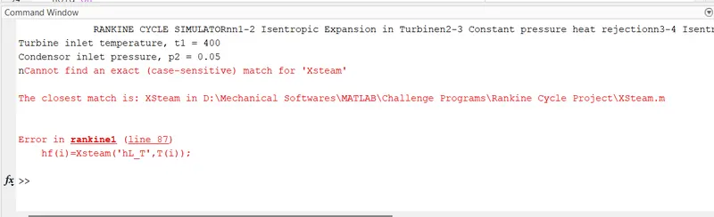
In line 87 I wrote XSteam as Xsteam.
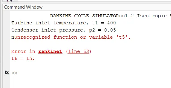
In line 63 I wrote t5 as ts.
Most of the Errors were small typos I made during programming.

RESULTS:

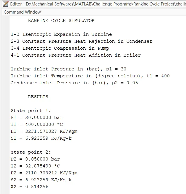
Results shown in the Command Window:

Results of the Plots:

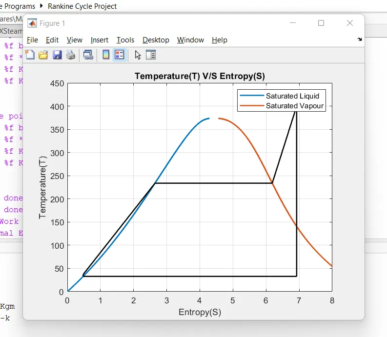
In the above graph, we see that from point 1 cycle started with the turbine, here dry saturated steam from the boiler was used to run the turbine. heat is rejected in this process so temperature decreased from t1 to t2. Then in the condenser, the steam is converted into a saturated liquid (water) that is t2 to t3 at constant pressure as the line is under the saturated curve. Water is forced by the pump to the boiler. here pressure is increased from p3 to p4. In the boiler water is converted into dry saturated steam that is t4 to t1 at constant pressure and then rotated by the turbine. As temperature decreases entropy also decreased and when increased entropy also increased so the entropy is dependent on temperature. The turbine work here is more than pump work always in the cycle. The pump work is very small in this cycle.
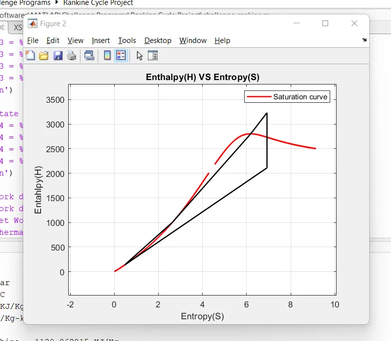
In the above graph, we can see when pressure increased enthalpy also increased and when decreased the enthalpy also decreased, also Same for the entropy when temperature increased entropy also increased and when decreased the entropy also decreased So, we can say that enthalpy and entropy totally depend on temperature and pressure. In the turbine (1-2) pressure decreased so enthalpy also decreased at constant entropy. In condenser (2- 3) temperature and pressure decreased so entropy and enthalpy also decreased. In the pump (3-4) very small change in temperature and pressure increase. So the entropy and enthalpy change are also very small. But in the boiler (4-1) temperature increased so the entropy also increased and practically when the temperature is increased pressure also increased in the cycle so entropy and enthalpy also increased simultaneously.

CONCLUSION:

We can conclude that the MATLAB program for Rankine cycle computed and this code helps to design the power plant operating condition by which the plant efficiency can be increased and specific steam consumption can be decreased.

REFERENCES:

Rankine cycle Simulator using MATLAB.

Ship work like this
in your own course.

Talk to a career counsellor

Ship work like thisin your own course.

Talk to a career counsellor

Ship work like this
in your own course.