Project 2 - Rankine cycle Simulator

Aim- write a code to Simulate the Rankine cycle for the given input parameters using MATLAB.

Rankine cycle-

The Rankine cycle is an idealized thermodynamic cycle describing the process by which certain heat engines, such as steam turbines or reciprocating steam engines, allow mechanical work to be extracted from a fluid as it moves between a heat source and heat sink. The Rankine cycle is named after, William john Macquorn Rankine a Scottish polymath professor at Glasgow University.

Heat energy is supplied to the system via a boiler where the working fluid (typically water) is converted to a high-pressure gaseous state (steam) in order to turn a turbine After passing over the turbine the fluid is allowed to condense back into a liquid state as waste heat energy is rejected before being returned to the boiler, completing the cycle. Friction losses throughout the system are often neglected for the purpose of simplifying calculations as such losses are usually much less significant than thermodynamic losses, especially in larger systems.

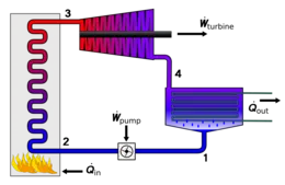
Where-

(1-2)isentropic compression
(2-3)constant pressure heat addition
(3-4)isentropic expansion
(4-1)constant pressure heat rejection

writing of code-

%progrem to calculate the net work output and work back ratio

clear all
close all
clc

%rankine cycle and simulate the t-s and h-s plot

fprintf('RANKINE CYCLE SIMULATOR\n')
fprintf('process 1-2 Isometric compression in the Pumpn \n');
fprintf('process 2-3 Constant pressure heat addition by Boilern\n');
fprintf('process 3-4 Isentropic expansion in the Turbinen\n');
fprintf('process 4-1 Constent pressure heat rejection by the Condensern\n');

%getting the user inputs

T3=input('Enter turbine inlet temperature in (Celcius)\n');
p3=input('Enter turbine inlet pressure in (bar)\n');
p4=input('Enter turbine outlet pressure in (bar)\n');


%process

%1-2 isentropic compression
%2-3 constant pressure heat addition
%3-4 isentropic expansion
%4-1 constent pressure heat rejection

%calculating enthalpy at pt.3
h3=XSteam('h_pT',p3,T3);

%calculating enthalpy at pt.1
hf1=XSteam('hL_p',p4);

%calculating enthalpy at pt.3
s3=XSteam('s_pT',p3,T3);

%as the line 3-4 is isentropic
s4=s3;

%calculating entropy at pt.1
sf1=XSteam('sL_p',p4);

%calculating entropy at diff at 0.005 bar
sfg4=XSteam('sV_p',p4)-XSteam('sL_p',p4);

% calculating quality of steam at pt.4
X=(s4-sf1)/sfg4;

%calculating Enthalpy at diff at 0.005 bar
hfg4=XSteam('hV_p',p4)-XSteam('hL_p',p4);

%Enthalpy at pt.4
h4=hf1+(X*hfg4)
%work out at turbine
Wt=h3-h4;

%specific volume at ppt.1
vf=XSteam('vL_p',p4);

%work consumed by pump
Wp=vf*(p3-p4);

%total work output
Wnet=Wt-Wp;

%enthalpy at saturation liquid of pt.2
hf2=Wp+hf1;

%input heat to the boiler
Qh=h3-hf2;

%efficiency of cycle
eff=(Wnet/Qh)*100;

%back work of the ratio
bac=Wp/Wt;

%properties at pt.1
T1=XSteam('Tsat_p',p4);
p1=p4;
h1=hf1;
s1=sf1;

%properties at pt.2
T2=XSteam('T_ps',p3,s1);
p2=p3;
h2=XSteam('h_ps',p3,s1);
s2=s1;

%properties at pt.3
T3;
p3;
h3;
s3;

%properties at pt.4
T4=XSteam('T_ph',p4,h4);
p4;
h4;
s4;

% properties of intermidiate pts. between process2-3
T5=XSteam('Tsat_p',p3);
p5=p3;
h5=XSteam('hL_p',p3);
s5=XSteam('sL_p',p3);
T6=XSteam('Tsat_p',p3);
p6=p3;
h6=XSteam('hV_p',p3);
s6=XSteam('sV_p',p3);

%output
fprintf('-------------RESULTS-------------\n');

fprintf('properties at point 1:\n');
fprintf('T1 = %f  Celciusn', T1);
fprintf('p1 = %f barn',p1);
fprintf('h1 = %f kj/kgn',h1);
fprintf('s1 = %f  kj/kg Cn',s1);

fprintf('properties at point 2:\n');
fprintf('T2 = %f  celciusn', T2);
fprintf('p2 = %f barn',p2);
fprintf('h2 = %f kj/kgm',h2);
fprintf('s2 = %f  kj/kg Cn',s2);

fprintf('properties at point 3:\n');
fprintf('T3 = %f  celciusn', T3);
fprintf('p3 = %f barn',p3);
fprintf('h3 = %f kj/kgm',h3);
fprintf('s3 = %f  kj/kg Cn',s3);

fprintf('properties at point 4:\n');
fprintf('T4 = %f  celciusn', T4);
fprintf('p4 = %f barn',p4);
fprintf('h4 = %f kj/kgm',h4);
fprintf('s4 = %f  kj/kg Cn',s4);

fprintf('net work output is %f kj\n',Wnet);
fprintf('Efficiency of cycle is %f %%n',eff);
fprintf('Back work ratio is %f n',bac);

% plotting T-s and h-s

%ploting saturation lines
T=(1:2000);

%loop to store values
for i=1:1:2000
    sL(1,i)=XSteam('sL_T',i);
    sV(1,i)=XSteam('sV_T',i);
    hL(1,i)=XSteam('hL_T',i);
    hV(1,i)=XSteam('hV_T',i);
end

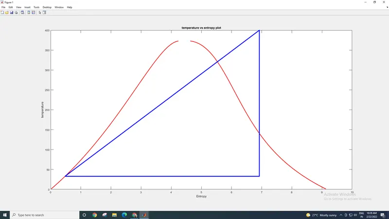
figure(1)
plot(sL,T,'r','linewidth',2);
hold on
plot(sV,T,'r','linewidth',2);
xlabel('Entropy');
ylabel('temperature');
title('temperature vs entropy plot');

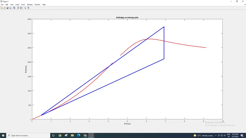
figure(2)
plot(sL,hL,'r','linewidth',2);
hold on;
plot(sV,hV,'r','linewidth',2);
xlabel('Entropy');
ylabel('Enthalpy');
title('Enthalpy vs entropy plot');


%ploying the rankine cycle
figure(1)
plot([s1,s2,s3,s4,s1],[T1,T2,T3,T4,T1],'b','linewidth',3);

figure(2)
plot([s1,s2,s3,s4,s1],[h1,h2,h3,h4,h1],'b','linewidth',3);

code explanation-

• to get started we have to open a new file
• whenever we start a new program it is good practice to include some commands
• input variables are taken
• properties such as temperature(T), pressure(p), enthalpy(h) and entropy(s) is found at each point of the cycle using some relations Xsteam library in MATLAB.
• As process 2-3 is isobaric so p2=p3
• As process 4-1 is also isobaric sop4=p1
• As process 3-4 is isentropic so s3=s4
• As process 1-2 is also isentropic so s1=s2
• in the steam table if the point is between liquid and vapour saturation lines then s(n)=sL(n)=XsV(n)

1. here n is the point number
2. s is entropy but we can use it for any number
3. sL(n) is liquid saturation entropy at point n
4. sV(n) is the vapour saturation at point n and X is the quality of stem at point n

• the same method is used for enthalpy h
• then we calculate the required output properties
• after calculating the required outputs the results are displayed
• then the t-s and h-s are plotted using the plot command

output-

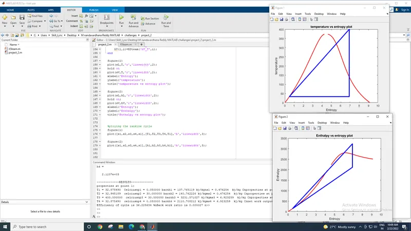
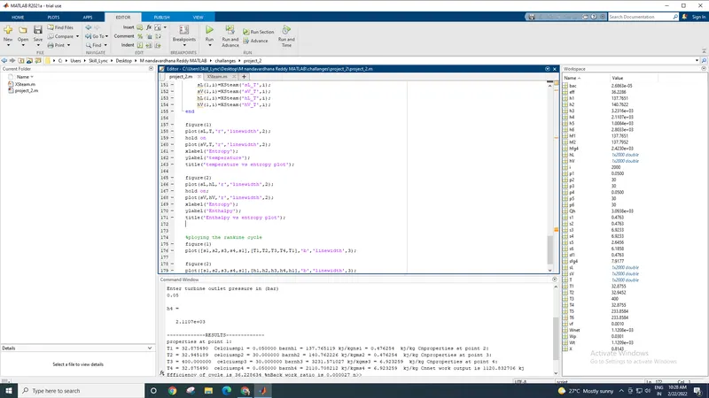
plots