Project 2 - Rankine cycle Simulator

Aim:

• To simulate basic Rankine Cycle

Objective:

1. Creating a Rankine Cycle Simulator using OCTAVE/MATLAB. Calculating the state points of the Rankine Cycle based on user inputs.
2. Then plotting the corresponding T-S and H-S plots for the given set of inputs.

Rankine cycle:

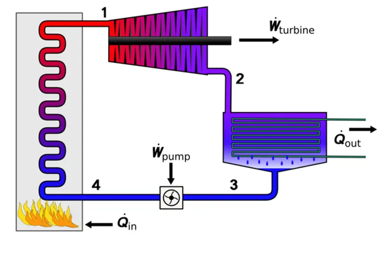
The different processes here are:

• Process 1-2: Isentropic Expansion in the turbine
• Process 2-3: Isobaric Heat Rejection by the condenser
• Process 3-4: Isentropic Compression in the pump
• Process 4-1: Isobaric Heat Addition by the boiler

Here the given inputs values are:

• Turbine inlet temperature = 400 C
• Turbine Inlet Pressure = 30 bars
• Turbine Outlet Pressure = 0.05 bars = Condenser Inlet Pressure

Program:-

clear all
close all
clc

% inputs 
disp('Rankine Cycle Simulator')
disp('1-2 corresponds to isentropic expansion in turbine')
disp('2-3 corresponds to constant pressure heat rejection in condenser')
disp('3-4 corresponds to isentropic compression in pump')
disp('4-1 corresponds to constant pressure heat addition in boiler')
fprintf('n')

p1 = input('Enter the pressure at the inlet of turbine (bar):');
t1 = input('Enter the temp at the inlet of the turbine (degree C):');
p2 = input('Enter the pressure at the inlet of condensor (bar):');

% At state point 1

h1 = XSteam('h_pT',p1,t1);
s1 = XSteam('s_pT', p1, t1);
%Since 1-2 is isentropic process

s2 = s1;

sf2 = XSteam('sL_p', p2);
sg2 = XSteam('sV_p', p2);
sfg2 = (sg2 - sf2);
%Finding dryness fraction (s2 = sf2 + x2* sfg2)
x2 = (s2 - sf2)/sfg2;
x2<1;
disp('Steam is wet at the inlet of the condenser')
fprintf('n')

%Finding Enthalpy
hf2 = XSteam ('hL_p',p2);
hg2 = XSteam ('hV_p',p2);
hfg2 = hg2 - hf2;
h2 = hf2 + x2*hfg2;
t2 = XSteam('Tsat_p',p2);

%Workdone by Turbine
wt = h1 - h2;

%Workdone by Turbine
wt = h1 - h2;

%For state point 3

%Work done by pump
p3 = p2;
vf3 = XSteam('vL_p',p3);
v3 = vf3;
wp = v3*(p1 - p2)*100;
t3 = XSteam('Tsat_p',p2);
h3 = XSteam('hL_p', p2);
s3 = XSteam('sL_p',p2);
%At point 4
p4 = p1;
h4 = wp + h3;

t4 = XSteam('T_ph',p4, h4);

s4 = s3; 
%Heat supplied to boiler 
qs = h1 - h4; 

%Heat Rejected by condenser 
qr = h2 - h3; 

%Work ratios and efficiency of turbine 

w_net = wt - wp; 
net_work_ratio = w_net/wt; 
efficiency = w_net/qs; 

%back work ratio 
back_work_ratio = wp/wt; 

%Specific Steam Consumption 
SSC = 3600/w_net; 
tf_sat = XSteam('Tsat_p',p1); 
sf_sat = XSteam('sL_p',p1); 
hf_sat = XSteam('hL_p',p1); 
sg_sat = XSteam('sV_p',p1); 
hg_sat = XSteam('hV_p',p1); 
%Plotting saturation liquid and vapour lines 

temp_range = linspace(1,373,1000); 
for i = 1:length(temp_range) 
S_L(i) = XSteam('sL_T',temp_range(i)); 
S_V(i) = XSteam('sV_T', temp_range(i)); 
end 

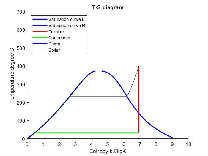
%Plotting T-S diagram 
figure(1) 
hold on 
plot(S_L,temp_range,'b','LineWidth',2) 
plot(S_V,temp_range,'b','LineWidth',2) 
plot([s1 s2], [t1 t2],'r','LineWidth',2) 
plot([s2 s3], [t2 t3],'g','LineWidth',2) 
plot([s3 s4], [t3 t4],'b','LineWidth',2) 

%Plotting curved constant pressure line 3 to 4 
t_cons_p = linspace(t4, XSteam('Tsat_p',p1),30); 
for i = 1:length(t_cons_p) 
S(i) = XSteam('s_pt',p1,t_cons_p(i)); 
end 
plot(S,t_cons_p,'k') 

t0_cons_p = linspace(XSteam('Tsat_p',p1),t1,300); 
for i=1:length(t0_cons_p) 
S0(i)=XSteam('s_pt',p1,t0_cons_p(i)); 
end 
plot(S0,t0_cons_p,'k') 

%Plotting the straight line of the phase change region 

plot([sf_sat sg_sat], [tf_sat tf_sat], 'k') 
title('T-S diagram') 
xlabel('Entropy kJ/kgK') 
ylabel('Temperature degree C') 
axis([0 10 0 700]) 
legend('Saturation curve L', 'Saturation curve R', 'Turbine', 'Condenser', 'Pump', 'Boiler', 'location','northwest') 

%Plotting H-S diagram 

figure(2) 
hold on 

%Plotting saturation curves 
temp_range1 = linspace(1, 373, 1000); 
for i=1:length(temp_range1) 
H_L1(i) = XSteam('hL_T', temp_range1(i)); 
H_V1(i) = XSteam('hV_T', temp_range1(i)); 
end 
plot(S_L, H_L1,'b','LineWidth',2) 
plot(S_V, H_V1,'b','LineWidth',2) 
plot([s1 s2], [h1 h2],'r','LineWidth',2) 
plot([s2 s3], [h2 h3],'g','LineWidth',2) 
plot([s3 s4], [h3 h4],'r','LineWidth',2) 

%For plotting the line between the pump and boiler 
s_pump = linspace(s3, s1, 1000); 
for i =1:length(s_pump) 
h_pump(i)=XSteam('h_ps',p1,s_pump(i)); 
end 
plot(s_pump, h_pump, 'k') 
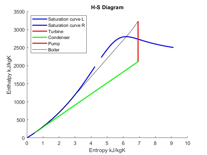
title('H-S Diagram') 
xlabel('Entropy kJ/kgK') 
ylabel('Enthalpy kJ/kgK') 
legend('Saturation curve L','Saturation curve R','Turbine','Condenser','Pump','Boiler','location','northwest') 

%Displaying the value of state point variables at each point
P_final = [p1 p2 p3 p4]; 
T_final = [t1 t2 t3 t4]; 
H_final = [h1 h2 h3 h4]; 
S_final = [s1 s2 s3 s4]; 
for i=1:4 
fprintf('At state point %d n', i) 
fprintf('Pressure p%d : %4.4f (bar) n',i,P_final(i)) 
fprintf('Temperature t%d : %4.4f (degree C) n',i,T_final(i)) 
fprintf('Enthalpy h%d : %4.4f (kJ/kgK) n',i,H_final(i)) 
fprintf('Entropy s%d : %4.4f (kJ/kg) n',i,S_final(i)) 
fprintf('n') 
end 
fprintf('The net work ratio is: %f n', net_work_ratio) 
fprintf('The back work ratio is: %f n', back_work_ratio) 
fprintf('The entered values are not valid as the steam is either Saturated or Super-saturated at the inlet of the condenser n') 
fprintf('Enter the valid values by running the program again n') 
return;

Command Window Output:

state point 1 nPressure p1 : 30.0000 (bar) n

Temperature t1 : 400.0000 (degree C) n

Enthalpy h1 : 3231.5710 (kJ/kgK) n

Entropy s1 : 6.9233 (kJ/kg) nnAt state point 2 n

Pressure p2 : 0.0500 (bar) n

Temperature t2 : 32.8755 (degree C) n

Enthalpy h2 : 2110.7082 (kJ/kgK) n

Entropy s2 : 6.9233 (kJ/kg) nn

At state point 3 nPressure p3 : 0.0500 (bar) n

Temperature t3 : 32.8755 (degree C) n

Enthalpy h3 : 137.7651 (kJ/kgK) n

Entropy s3 : 0.4763 (kJ/kg) nn

At state point 4 nPressure p4 : 30.0000 (bar) n

Temperature t4 : 32.9639 (degree C) n

Enthalpy h4 : 140.7761 (kJ/kgK) n

Entropy s4 : 0.4763 (kJ/kg) nn

The net work ratio is: 0.997314 n

The back work ratio is: 0.002686

Outputs:

1. T-S diagram:

2. H-S diagram