Project 2 - Rankine cycle Simulator

The program indicates the rankline cycle plot

clear all
close all
clc

%Information
fprintf('n RANKINE CYCLE SIMULATOR');
fprintf('nn1-2 Isentropic Expansion in turbine');
fprintf('n2-3 Constant Pressure Heat Rejection in thr Condenser');
fprintf('n3-4 Isentropic compression in pump ');
fprintf('n4-1 Constant Pressure Heat Addition by the Boilers');

%Inputs
p1=input('Pressure at the Turbine inlet (bar) : ');
t1=input('Temperature ar the turbine inlet (celsius) : ');
p2=input('Pressure at the Condenser : ');

% @ stage1 turbine inlet
% p1 & t1 are given
h1=XSteam('h_pT',p1,t1);
s1=XSteam('s_pT',p1,t1);

% @ stage 2 Condenser Inlet 
%p2 is given 
s2=s1;
sf2=XSteam('sL_p',p2);
sg2=XSteam('sV_p',p2);
hf2=XSteam('hL_p',p2);
hg2=XSteam('hV_p',p2);
x2=(s2-sf2)/(sg2-sf2);
h2=hf2+(x2*(hg2-hf2));

% @ stage 3 pump Inlet
p3=p2;
h3=XSteam('hL_p',p3);
s3=XSteam('sL_p',p3);
t3=XSteam('Tsat_p',p3);
t2=t3;

% @ stage 4 Boiler Inlet
p4=p1;
s4=s3;
h4=XSteam('h_ps',p4,s4);

cp4=XSteam('Cp_ps',p4,s4);
cv4=XSteam('Cv_ps',p4,s4);
lambda=cp4/cv4;
t4=t3/((p3/p4)^((lambda-1)/(lambda)));

t5=XSteam('TSat_p',p1);
t6=t5;
s5=XSteam('sL_p',p1);
s6=XSteam('sV_p',p1);
h5=XSteam('hL_p',p1);
h6=XSteam('hV_p',p1);


%Turbine work
Wt=h1-h2;

%Pump work
Wp=h4-h3;

%Net work (KJ/Kg)
W=Wt-Wp;

%Heat in & out of the system
Q_in=h1-h1;
Q_out=h2-h3;

%Thermal Efficiency
ntherm=(W/Q_in)*100;

%steam rate (kg/KWh)
SSC=3600/W;

%Back Work Ratio
BWR=(h1-h4)/(h2-h3);

%to plot Saturation Curve
T =linspace(1,400,500);
for i=1:length(T)
    h_l(i)=XSteam('hL_T',T(i));
    h_v(i)=XSteam('hV_T',T(i));
    s_l(i)=XSteam('sL_T',T(i));
    s_v(i)=XSteam('sV_T',T(i));
end

%plotting TS diagram
figure(1)
hold on
plot([s1 s2],[t1 t2],'linewidth',3,'color','b')
plot([s2 s3],[t2 t3],'linewidth',3,'color','b')
plot([s3 s4],[t3 t4],'linewidth',3,'color','b')
plot([s4 s5],[t4 t5],'linewidth',3,'color','b')
plot([s5 s6],[t5 t6],'linewidth',3,'color','b')
xlabel('Entropy (KJ/Kgk');
ylabel('Temperature (deg C)');
s_1=linspace(s6,s1,500);
for j=1:length(s_1)
    t_1(j)=XSteam('T_ps',p1,s_1(j));
end
plot(s_1,t_1,'linewidth',3,'Color','b')
plot(s_l,T,'linewidth',1.5,'Color','r')
plot(s_v,T,'linewidth',1.5,'Color','r')

%Annotations
text(s1,t1,'1','FontSize',15);
text(s2,t2,'2','FontSize',15);
text(s3,t3,'3','FontSize',15,'VerticalAlignment','top')
text(s4,t4,'4','FontSize',15,'VerticalAlignment','bottom')
text(s5,t5,'5','FontSize',15,'VerticalAlignment','bottom')
text(s6,t6,'6','FontSize',15,'VerticalAlignment','bottom')

figure(2)
hold on
title('H-S diagram')
plot([s1 s2],[h1 h2],'LineWidth',2,'Color','b')
plot([s2 s3],[h2 h3],'LineWidth',2,'Color','b')
plot([s3 s4],[h3 h4],'LineWidth',2,'Color','b')


h_4=linspace(h4,h5,500);
for k=1:length(h_4)
    s_4(k)=XSteam('s_ph',p1,h_4(k));
end

h_6=linspace(h6,h1,500);
for k=1:length(h_6)
    s_6(k)=XSteam('s_ph',p1,h_6(k));
end

plot(s_4,h_4,'LineWidth',2,'Color','b')
plot([s5 s6],[h5 h6],'LineWidth',2,'Color','b')
xlabel('Specific Entropy (KJ/Kgk)')
ylabel('Specific Enthalpy (kJ/kg)')
plot(s_l,h_l,'LineWidth',1.5,'Color','b')
plot(s_v,h_v,'LineWidth',1.5,'Color','b')

%Annotations
text(s1,h1,'1','FontSize',15);
text(s2,h2,'2','FontSize',15);
text(s3,h3,'3','FontSize',15,'VerticalAlignment','top')
text(s4,h4,'4','FontSize',15,'VerticalAlignment','bottom')
text(s5,h5,'5','FontSize',15,'VerticalAlignment','bottom')
text(s6,h6,'6','FontSize',15,'VerticalAlignment','bottom')

%Resulr Window
fprintf('nRESULTSnn');
fprintf('At State Point 1:n');
fprintf('P1=%f Barn',p1);
fprintf('T1=%f Deg Celsius',t1);
fprintf('H1=%f KJ/Kgn',h1);
fprintf('S1=%f KJ/Kgknn',s1);

fprintf('At State Point 2:n');
fprintf('P2=%f Barn',p2);
fprintf('T2=%f Deg Celsius',t2);
fprintf('H2=%f KJ/Kgn',h2);
fprintf('S2=%f KJ/Kgknn',s2);

fprintf('At State Point 3:n');
fprintf('P3=%f Barn',p3);
fprintf('T3=%f Deg Celsius',t3);
fprintf('H3=%f KJ/Kgn',h3);
fprintf('S3=%f KJ/Kgknn',s3);

fprintf('At State Point 4:n');
fprintf('P4=%f Barn',p4);
fprintf('T4=%f Deg Celsius',t4);
fprintf('H4=%f KJ/Kgn',h4);
fprintf('S4=%f KJ/Kgknn',s4);

fprintf('Work done by Turbine is : %f KJ/Kgn',Wt);
fprintf('Work done by Pump is : %f KJ/Kgn',Wp);
fprintf('Net Work done on the System : %f KJ/kgn',Wp);
fprintf('Specific Steam Consumption is : %f kg/KWhn',SSC);
fprintf('The Net Thermal Efficiency of the System is : %fn',ntherm);
fprintf('The BWR of the Rankine Cycle is found to be : %fn',BWR);

Explanation:

We start the program using close all clear all clc. we given the information using fprintf series of words are been given now input the values in the command windows p1 t2 and p2.

For the stage 1 turbine inlet the pressure and temperature are p1 and t1 we use the XSteam h and s are enthalpy and entropy are given as h and s respectively. pressure iand temperature is p1 t1.

For stage 2 Condenser Inlet the pressure is p2 in the XSteam we use sf2 hf2 sg2 hg2 they are enthalpy (h) and specific heat (s) of the saturated temperature at two different pressure.To calculate x2 the formula is (s2-sf2)/(sg2-sf2) and for h2 is hf2+(x2*(hg2-hf2)) respectively.

For stage three pump inlet in this point p3 and p2 are equal so we need to calculate h3 s3 and t3 where when p2 is same as p3 then temperature is also same t2 is equal to t3 is as similkar as stage 2.

For stage 4 Boiler inlet the pressure p1 = p4,s4 = s3 we calculate the t5,t6,s5,s6,h5 and h6 for the fourth stage

Formulas to calculate the following:

Turbine work
Wt=h1-h2

Pump work
Wp=h4-h3

Net work (KJ/Kg)
W=Wt-Wp

Heat in & out of the system
Q_in=h1-h1
Q_out=h2-h3

Thermal Efficiency
ntherm=(W/Q_in)*100

steam rate (kg/KWh)
SSC=3600/W

Back Work Ratio
BWR=(h1-h4)/(h2-h3)

The next step is to plot the saturation curve the linspace command (1,400,500) the values are been printed we use the for loop for the function i=1:lenght of T,we calculate the h_l,h_v,s_V and s_l respectively.

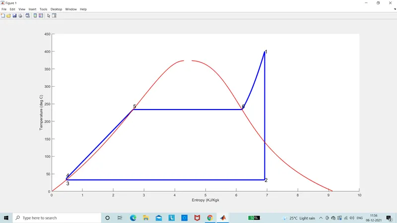
Now, plotting the TS diagram starting with the hold on command using s1 to s6 respectivelt similarly for t1 to t6 xlabel is Entropy and ylabel is Temperature respectively,we use for loop an d give the line iwdth for the plot and annotations for the text like font size and vertical alignment to align it and top and bottom to align at the exact position.

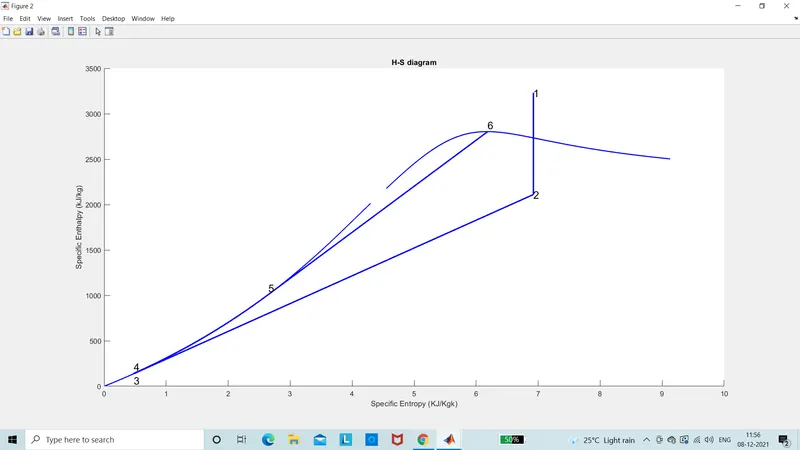
We now plot fot the HS diagram we use as similar fot he the ts diagram we use a for loop and the annotations in this case we use s4 and h4 to plot

The step is to print the following in the result window so that the calculate turbine work pump work etc are been calculated and displayed respectively we use fprintf command for the required operation.

Errors:

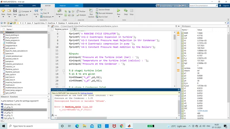
the XSteam file was not in the required directory

Result:

T-S diagram

H-S diagram