Project 2 - Rankine cycle Simulator

RANKINE CYCLE SIMULATOR

Simple Rankine Cycle

• Rankine cycle consists of certain predefined thermodynamic processes which in symphony produces power by utilising an energy-dense chemical reagent for energy input.
• The cycle is used mainly in Steam Powerplant. Where the working fluid is superheated steam, which is used to run the turbine and useful work gets generated by the expansion process of the steam.
• The different processes are given below
• 
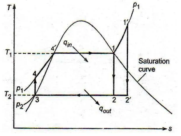
  1. Process 1-2 is an Isentropic expansion that takes place in the turbine.
  2. Process 2-3 is an Isobaric heat dissipation in the condenser.
  3. Process 3-4 is an Isentropic compression, where the pump pressurizes the liquid water to high pressure.
  4. Process 4-1 is an Isobaric heat addition process that takes place inside the boiler and steam generator.
• The Rankine cycle is the cycle that steers the production of energy from the steam powerplant plant. The reason to use the Rankine cycle is to maximize the work output and reduce the input power. The input power is less due to the pressure of water being increased in liquid which reduces the pressurizing power required as the liquid state of water is noncompressible.
• Ideal Rankine Cycle is the simple Rankine cycle that generates power in simple four thermodynamic processes, where many ideal conditions are assumed to keep the calculations simple and conveyable.
• The turbine inlet state is always maintained in the superheated state to increase the life span of the turbine blades as the dryness ratio doesn't fall drastically. Which ensures the longevity of the blade.
• Assumptions are as follows
  • Both pump and turbine don't work isentropically in reality. So the work generated in reality is less than the ideal turbine work similarly the work input given to the pump, in reality, is greater than the ideal one.
  • The constant pressure heat addition process is not that accurate in reality there is a slight increase in pressure while the heat is added to the water in the process of steam generation.
  • To neglect these intrinsic inefficiencies we consider the ideal scenario and try to learn the simple version of the Rankine cycle.

• Matlab code for the Rankine Cycle Simulator

  • %% Rankine Cycle simulator
    
    clear all
    close all
    clc
     
    %% Step1
    
    % Defining Deg Celcius to Kelvin conversion factor
    k=273.15;
    % Turbine inlet temperature is defined 
    t1=input('Enter the Inlet temperature for turbine(in Deg Celcius) is =');
    T1=t1+k;
    % Inlet pressure of steam for turbine is defined
    p1=input('Enter the Inlet pressure for turbine (in Bar) is= ');
    
    
    %% Step2
    
    % State point 1
    T1=t1+k;
    % Extracting h1 and s1 from XSteam function
    h1 = XSteam('h_pT',p1,t1);
    s1 = XSteam('s_pT',p1,t1);
    
    % State point 2
    % Evaluating turbine outlet state point
    p2=input('Enter the Outlet pressure for turbine (in Bar) is =');
    t2=XSteam('Tsat_p',p2);
    T2=t2+k;
    % Extracting s2 and h2 from Xsteam function
    % For simple Rankine Cycle the 1-2 process is isentropic process
    s2=s1;
    % Evaluating enthalpy at turbine outlet
    h2=XSteam('h_ps',p2,s2);
    % Evaluating dryness factor at end of turbine
    x=XSteam('x_ps',p2,s2);
    
    
    % State point 3
    % Evaluating for condenser outlet
    % Condenser works at same pressure as the outlet of Turbine
    p3=p2;
    % The 2-3 process is a isobaric heat dissipation the temperature remains
    % same as the latent heat changes to heat dissipation
    t3=t2;
    T3=t3+k;
    % Evaluating enthalpy at end of condenser
    h3=XSteam('hL_p',p2);
    % Evaluating entropy at end of condenser
    s3=XSteam('sL_p',p2);
    
    % State point 4
    % Evaluating for pump outlet
    % Pump pressurises the the saturated liquid water to subcooled water by an
    % insentropic process
    p4=p1;
    s4=s3;
    % Temprature of the subcooled water
    t4=XSteam('T_ps',p4,s4);
    T4=t4+k;
    % Evaluating enthalpy of subcooled wated
    h4=XSteam('h_ps',p4,s4);
    
    % State point 5
    % Evaluating Saturated liquid state points at p1
    t5=XSteam('Tsat_p',p1);
    T5=t5+k;
    s5=XSteam('sL_p',p1);
    h5=XSteam('hL_p',p1);
    
    % State point 6
    % Evaluating Saturated vapour state points at p1
    T6=T5;
    s6=XSteam('sV_p',p1);
    h6=XSteam('hV_p',p1);
    
    %% Step3
    
    % Heat added in kJ/kg
    q_in=h1-h4
    % Pump work calculation in kJ/kg
    % w_p=h4-h3
    vl_c=XSteam('vL_p',p2);
    w_p=vl_c*(p1-p2)*100
    % Turbine work calculation in kJ/kg
    w_t=h1-h2
    w_net=w_t-w_p
    % Efficiency of Rankine Cycle
    eff=(w_t-w_p)*100/q_in
    % Back Work Ratio w_p/w_t;
    bwr=w_p/w_t
    
    %% Step4
    
    t_l=linspace(0,374,1000);
    T_l=t_l+k;
    t_v=linspace(374,0,1000);
    T_v=t_v+k;
    
    %% Step5
    
    for j=1:length(t_l)
    
        % Evaluating credentials for plotting Vapour dome in T-s Plane        
        % Evaluating credentials for plotting Vapour dome in h-s Plane
        % Evaluating Liquid Saturation Enthalpies
        h_l(j)= XSteam('hL_T',t_l(j));
        % Evaluating Liquid Saturation Entropies
        s_l(j)=XSteam('sL_T',t_l(j));
        % Evaluating Vapour Saturation Enthalpies
        h_v(j)=XSteam('hV_T',t_v(j));
        % Evaluating Vapour Saturation Entropies
        s_v(j)=XSteam('sV_T',t_v(j));
    end
    
    %% Step6
    
    % Plots
    % First figure window
    figure(1)
    % T-s plot of the Rankine cycle
    plot([s1 s2],[T1 T2],[s2 s3],[T2 T3],[s3 s4],[T3 T4],[s4 s5],[T4 T5],[s5 s6],[T5 T6],[s6 s1],[T6 T1],'linewidth',2,'color','[0 0 0]')
    
    hold on
    
    % Marking the state points
    plot(s1,T1,'marker','o','MarkerSize',9,'color','r')
    plot(s2,T2,'marker','o','MarkerSize',9,'color','r')
    plot(s3,T3,'marker','o','MarkerSize',9,'color','r')
    plot(s4,T4,'marker','o','MarkerSize',9,'color','r')
    plot(s5,T5,'marker','o','MarkerSize',9,'color','r')
    plot(s6,T6,'marker','o','MarkerSize',9,'color','r')
    
    % Plotting saturation lines
    plot(s,T_l,'linewidth',2,'color','g')
    plot(s_v,T_v,'linewidth',2,'color','g')
    % Labelling the plot figure
    title('VAPOUR DOME AND RANKINE CYCLE IN T-s PLANE')
    xlabel('ENTROPY (kJ/kg-K)')
    ylabel('TEMPERATURE (K)')
    
    %% Step7
    
    % To represent each state points of the plot we use gtext command
    % It is important to start the naming from the superheated point in figure
    % window 
    gtext('1')
    gtext('2')
    gtext('3')
    gtext('4')
    gtext('5')
    gtext('6')
    % Mentioning saturation lines
    gtext('SATURATION VAPOUR LINE')
    gtext('SATURATION LIQUID LINE')
    
    hold off
    
    %% Step8
    
    % Second figure window
    figure(2)
    % h-s plot of the Rankine cycle
    plot([s1 s2],[h1 h2],[s2 s3],[h2 h3],[s3 s4],[h3 h4],[s4 s5],[h4 h5],[s5 s6],[h5 h6],[s6 s1],[h6 h1],'linewidth',2,'color','[0 0 0]')
    
    hold on
    
    % Marking the state points
    plot(s1,h1,'marker','o','MarkerSize',9,'color','r')
    plot(s2,h2,'marker','o','MarkerSize',9,'color','r')
    plot(s3,h3,'marker','o','MarkerSize',9,'color','r')
    plot(s4,h4,'marker','o','MarkerSize',9,'color','r')
    plot(s5,h5,'marker','o','MarkerSize',9,'color','r')
    plot(s6,h6,'marker','o','MarkerSize',9,'color','r')
    
    % Plotting saturation lines
    plot(s_l,h_l,'linewidth',2,'color','b')
    plot(s_v,h_v,'linewidth',2,'color','b')
    % Labelling the plot figure
    title('VAPOUR DOME AND RANKINE CYCLE IN h-s PLANE')
    xlabel('ENTROPY (kJ/kg-K)')
    ylabel('ENTHALPY (kJ/kg)')
    
    %% Step9
    % To represent each state points of the plot we use gtext command
    % It is important to start the naming from the superheated point in figure
    % window
    gtext('1')
    gtext('2')
    gtext('3')
    gtext('4')
    gtext('5')
    gtext('6')
    % Mentioning saturation lines
    gtext('SATURATION VAPOUR LINE')
    gtext('SATURATION LIQUID LINE')
    
    hold off
    
    %% Step10
    
    % Lines to show in the command window
    % Printing the heading in bold
    fprintf('                              <strong> RANKINE CYCLE SIMULATOR </strong> \n')
    % Printing the state processes bold
    fprintf('<strong> 1-2 is Isentropic Expansion in the Turbine </strong>\n')
    fprintf('<strong> 2-3 is Constant Pressure Heat Rejection by Condenser </strong>\n')
    fprintf('<strong> 3-4 is Isentropic Compression in the Pump </strong>\n')
    fprintf('<strong> 4-1 is Constant Pressure Heat Addition by the Boiler </strong>\n\n')
    % Printing the input statements in command window
    fprintf(' Enter Inlet temperature for turbine(in Degree Celcius) is = %f Deg Celcius \n',t1)
    fprintf(' Enter the Inlet pressure for turbine (in Bar) is= %f Bar \n',p1)
    fprintf(' Enter the Outlet pressure for turbine (in Bar) is= %f Bar \n\n',p2)
    
    %% Step11
    
    % Printing results in command window
    fprintf('                                  <strong> RESULTS </strong> \n')
    % Printing variables at state 1
    fprintf('At State point 1\n')
    fprintf(' T1 is : %f Deg Celcius \n',t1)
    fprintf(' P1 is : %f Bar \n',p1)
    fprintf(' H1 is : %f kJ/kg \n',h1)
    fprintf(' S1 is : %f kJ/kg*K \n\n',s1)
    % Printing variables at state 2
    fprintf('At State point 2\n')
    fprintf(' T2 is : %f Deg Celcius \n',t2)
    fprintf(' P2 is : %f Bar \n',p2)
    fprintf(' H2 is : %f kJ/kg \n',h2)
    fprintf(' S2 is : %f kJ/kg*K \n',s2)
    fprintf(' X2 is : %f \n\n',x)
    % Printing variables at state 3
    fprintf('At State point 3\n')
    fprintf(' T3 is : %f Deg Celcius \n',t3)
    fprintf(' P3 is : %f Bar \n',p3)
    fprintf(' H3 is : %f kJ/kg \n',h3)
    fprintf(' S2 is : %f kJ/kg*K \n\n',s3)
    % Printing variables at state 4
    fprintf('At State point 4\n')
    fprintf(' T4 is : %f Deg Celcius \n',t4)
    fprintf(' P4 is : %f Bar \n',p4)
    fprintf(' H4 is : %f kJ/kg \n',h4)
    fprintf(' S4 is : %f kJ/kg*K \n\n',s4)
    % Printing characteristics outputs of the Rankine cycle 
    fprintf('Rankine Cycle Properties\n')
    fprintf(' W_t is : %f kJ/kg\n',w_t)
    fprintf(' W_p is : %f kJ/kg\n',w_p)
    fprintf(' W_net is : %f kJ/kg\n',w_net)
    fprintf(' Thermal Eff is : %f %%\n',eff)
    fprintf(' B.W.R is : %f \n',bwr)
    

  • The matlab program is started from clear all, close all, and clc.
  • Step1
    
    • As defined in the problem statement, the input is recorded by the program by using input command. Using this syntax the user given inputs have been recorded for further use.
    • Input values are t1 and p1.
  • Step2
    • To extract every state point of the Rankine cycle using the input stored from the last step.
    • The process starts from state point 1, which is the turbine inlet. To get the state point we have to calculate the specific entropy and specific enthalpy of each state. After which we can locate the point in both h-s and T-s planes.
    • To get the h and s values of each state we have to make use of the steam table and call the function using function call % Extracting h1 and s1 from XSteam function XSteam.
    • By using the same procedure we can find the state points of turbine inlet, condenser input, pump input, pump output, saturated liquid at p1, and saturated vapour at p1.
  • Step3
    • After getting all the state points the next step is to calculate the heat added, turbine work output, required pump work, efficiency and back work ratio.
  • Step4
    • To create the vapour dome for T-s and h-s plot, the temperature range has been defined using the linspace command. Where two temperature arrays have been created for the saturated liquid line and saturated vapour line. T_l and T_v which are in kelvin scale.
  • Step5
    • Finding the values of the entropy and enthalpy for saturated liquid and vapour for the temperature range(defined above) using a for loop.
  • Step6
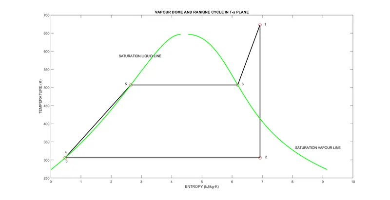
    • The 1st figure window has been created to plot T-s curves.
    • First, a plot has been created by connecting all six state points, which have been calculated in the above steps to make a Rankine Cycle in the T-s plane.
    • To distinguish each state point, a marker has been used.
    • Then the vapour dome has been plotted using the results from step4.
    • xlabel, ylabel and title has been added to the plot to make the figure window more appealing.
  • Step7
    • gtext command is used to add the state point numbers to the plot after the figure gets displayed.
    • By using the gtext command, saturated vapour line and saturated liquid line have been added to the plot.
  • Step8
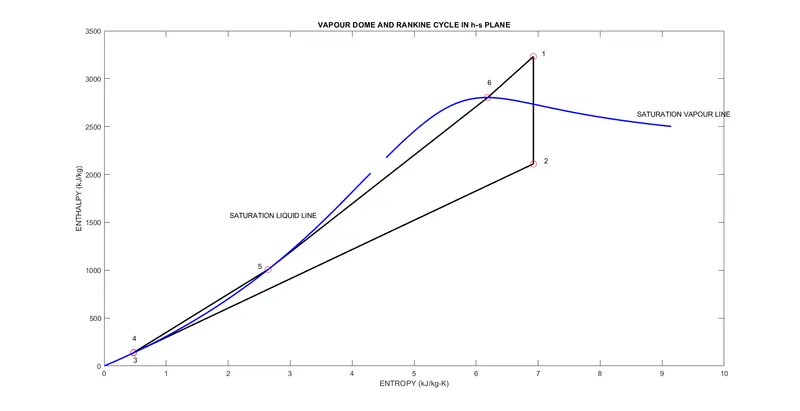
    • The 2nd figure window has been created to plot h-s curves.
    • First, a plot has been created by connecting all six state points, which have been calculated in the above steps to make a Rankine Cycle in h-s plane.
    • To distinguish each state point, a marker has been used.
    • Then the vapour dome has been plotted using the results from step4.
    • xlabel, ylabel and title has been added to the plot to make the figure window more appealing.
  • Step9
    • gtext command is used to add the state point numbers to the plot after the figure gets displayed.
    • By using the gtext command, saturated vapour line and saturated liquid line have been added to the plot.
  • Step10 (Printing statements in the command window)
    • The first line is to print the heading (RANKINE CYCLE SIMULATOR) in bold using ('<strong> </strong>') syntax.
    • Then printing the processes names in bold.
    • Then printing the input arguments to be displayed respectively which were stored before.
  • Step11 (Printing results in the command window)
    • The first line is to print the heading (RESULTS) in bold using ('<strong> </strong>') syntax.
    • Then printing state point variables at each state.
    • Finally displaying output from this analysis in the command window.
• Results
  • The printed T-s plot has been shown below
  • 
  • The h-s plot has been shown below
  • 
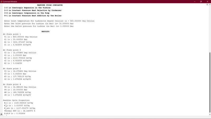
  • The printed output in command window of efficiency and back work ratio is given below,
  • 
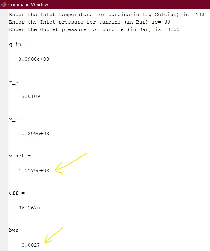
  • The simulator printed in command window is shown below
  • 
• Errors
  • I've encountered many errors while making progress in this project but it is very difficult to keep a track of it but here are some
  • 
  • I executed plots for h5, h6 which were not yet defined at that time. To overcome this I have to rearrange the code.
  • 
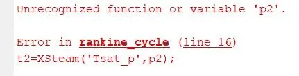
  • This error popped when I tried to use the undefined pressure p2.