Project 2 - Rankine cycle Simulator
Aim-To create rankine cycle simulator using Matlab.
objective -we have three inputs 1)turbine inlet temperature
2)turbine inlet pressure
3)turbine outlet pressure
Based on these three inputs calculate every state points properties, thermal efficiency of cycle using Matlab
and the T-S and h-S diagram
- to get the various properties use the XSteam library.
RANKINE CYCLE-IT IS THE THERMODYNAMIC CYCLE WHICH CONVERT PRESSURE ENERGY INTO THE MECHANICAL ENERGY WITH THE HELP OF WORKING SUBSTANCE AS WATER AND VAPOUR.
r
There are four components in the rankine cycle
1)boiler-it is the device used to create steam from the water,the process used here is the constant pressure heat addition to the water.
heat supplied(Qin)=h3-h2
2)turbine-it is used for extracting the work from the system,the process used here is the isentropic expansion.
work output(Wout)=h3-h4
3)condenser-the device used for removing the heat from the system with constant pressure heat rejection process
heat rejected(Qr)=h4-h1
4)pump-the pump is used for the pumping the fluid or the working substance to cycle
work input(Win)=h2-h1
here
h3=enthalpy at turbine inlet(KJ/kg)
h4=enthalpy at condenser inlet(KJ/kg)
h1=enthalpy at pump inlet(KJ/kg)
h2=enthalpy at boiler inlet(KJ/kg)
- the thermal efficiency is then calculated by `eta="net work output"/"heat supplied"="Wnet"/"Qsupplied"`
T-S diagram of the rankine cycle H-S diagram of rankine cycle
This is the ideal rankine cycle in which we did not consider the losses due to dissipative effects and the lack of perfect equilibrium.
main code
The symbol notation for the main code
h1=enthalpy at turbine inlet(KJ/kg)
h2=enthalpy at condenser inlet(KJ/kg)
h3=enthalpy at pump inlet(KJ/kg)
h4=enthalpy at boiler inlet(KJ/kg)
W12=work output of turbine in Kj/kg
W34=work input to the pump in KJ/kg
Q41=heat added in the system by boiler KJ/kg
Q23=heat rejection in the condensor KJ/kg
clear all
close all
clc

fprintf('\t\t\t\t\t\t\tRANKINE CYCLE SIMULATOR\t\t\t\t\n')
disp("")
fprintf('1-2 isentropic expansion in the turbine\n')
fprintf('2-3 constant pressure heat rejection in condensor\n')
fprintf('3-4 isentropic compression in pump\n')
fprintf('4-1 constant pressure heat addition in the boiler\n')
% units and the notation of quantities used in the code
% pressure(p)=bar
% temperature(T)=degree celsius
% specific entropy(s)= KJ/kg*K
% specific enthalpy(h)= KJ/kg
% specific heat at constant pressure(Cp)=KJ/kg*K
% specific volume(v)=m^3/kg

%state points at 1 /tubine inlet state points/
% taking the inputs from the user for the cycle
p1=input("enter the turbine inlet pressure(in bar)=");
T1=input("enter the turbine inlet temperature(in degree celcius)=");
p2=input("enter the pressure at condenser (in bar)=");

%p1=30
%T1=400
h1=XSteam('h_pT',p1,T1);
s1=XSteam('s_pT',p1,T1);
x1=XSteam('x_ph',p1,h1);
Cp1=XSteam('Cp_pT',p1,T1);

%state points 2
% condenser inlet points

s2=s1;
h2=XSteam('h_ps',p2,s2);
T2=XSteam('T_ps',p2,s2);
Cp2=XSteam('Cp_pT',p2,T2);
x2=XSteam('x_ph',p2,h2);

%state points 3
p3=p2;
s3=XSteam('sL_p',p3);
h3=XSteam('hL_p',p3);
v3=XSteam('vL_p',p3);
T3=XSteam('T_ps',p3,s3);
%state point 4
p4=p1;
s4=s3;
T4=XSteam('T_ps',p4,s4);


%all the work done and heat supplied is calculated in the KJ/kg


% work done by the turbine
% for process 1 to 2

W12=h1-h2;           %KJ/kg


% heat rejected by the condenser

Q23=h2-h3;    %KJ/kg

% work done by the pump
% for the process 3 to 4
%  W34=h4-h3;
W34=v3*(p4-p3)*100;
h4=W34+h3;

%heat added by the boiler
% for process 4 to 1
Q41=h1-h4;


% calculating the efficiency of the cycle
Wnet=W12-W34;
Qsupplied=Q41;
efficiency=(Wnet/Qsupplied)*100;

%specific steam consumption
ssc=3600/Wnet;      %kg/KJ

% calculating the back work ratio
% back work ratio=pump work/turbine work
 BWR=W34/W12;

fprintf("at state point 1\n");
fprintf("P1 is =%f in bars\n",p1);
fprintf("T1 is =%f in celcius\n",T1);
fprintf("S1 is =%f in KJ/kgKk\n",s1);
fprintf("H1 is =%f in KJ/kg\n",h1);
fprintf("\n")
disp("")
fprintf("at state point 2\n");
fprintf("P2 is =%f in bars\n",p2);
fprintf("T2 is =%f in celcius\n",T2);
fprintf("S2 is =%f in KJ/kgKk\n",s2);
fprintf("H2 is =%f in KJ/kg\n",h2);
fprintf("\n")
disp("")
fprintf("at state point 3\n");
fprintf("P3 is =%f in bars\n",p3);
fprintf("T3 is =%f in celcius\n",T3);
fprintf("S3 is =%f in KJ/kgKk\n",s3);
fprintf("H3 is =%f in KJ/kg\n",h3);
fprintf("\n")
disp("")
fprintf("at state point 4\n");
fprintf("P4 is =%f in bars\n",p4);
fprintf("T4 is =%f in celcius\n",T4);
fprintf("S4 is =%f in KJ/kgKk\n",s4);
fprintf("H4 is =%f in KJ/kg\n",h4);
fprintf("\n")
disp("")
fprintf("Wt is =%f in KJ/kg\n",W12);
fprintf("Wp is =%f in KJ/kg\n",W34);
fprintf("Wnet is =%f in KJ/kg\n",Wnet);
fprintf("thermal efficiency is =%f in KJ/kg\n",efficiency);
fprintf("specific dteam consumption is =%f in kg/KJ\n",ssc);
fprintf("back work ration is =%f \n",BWR);
%calculation points on the saturation graph
T6=XSteam('Tsat_p',p1);
s5=XSteam('sL_p',p1);
s6=XSteam('sV_p',p1);
h6=XSteam('hV_p',p1);
h5=XSteam('hL_p',p1);
T5=T6;
% plotting the saturation curve
T=linspace(1,400,1000);

for i=1:length(T)

    sf(i)=XSteam('sL_T',T(i));
    sg(i)=XSteam('sV_T',T(i));
    hf(i)=XSteam('hL_T',T(i));
    hg(i)=XSteam('hV_T',T(i));
end

%% ff
figure(1)
plot(sf,T,'b','linewidth',2)
hold on
plot(sg,T,'b','linewidth',2)
plot([s1 s2],[T1 T2],'r','linewidth',2)
plot([s2 s3],[T2 T3],'r','linewidth',2)

plot([s3 s4],[T3 T4],'r','linewidth',2)
plot([s4 s5],[T4 T5],'r','linewidth',2)
plot([s5 s6],[T5 T6],'r','linewidth',2)
plot([s6 s1],[T6 T1],'r','linewidth',2)
ylim([0 500])
text(s1,T1,'1','fontsize',20)
text(s2,T2,'2','fontsize',20)
text(s3,T3,'3','fontsize',20)
text(s4,T4,'4','fontsize',20)
xlabel('entropy')
ylabel('temperature')
title('T-S diagram rankine cycle')

figure(2)
plot(sf,hf,'b','linewidth',2)
hold on
plot(sg,hg,'b','linewidth',2)
plot([s1 s2],[h1 h2],'r','linewidth',2)
plot([s2 s3],[h2 h3],'r','linewidth',2)

plot([s3 s4],[h3 h4],'r','linewidth',2)
plot([s4 s5],[h4 h5],'r','linewidth',2)
plot([s5 s6],[h5 h6],'r','linewidth',2)
plot([s6 s1],[h6 h1],'r','linewidth',2)
ylim([0 4000])
text(s1,h1,'1','fontsize',20)
text(s2,h2,'2','fontsize',20)
text(s3,h3,'3','fontsize',20)
text(s4,h4,'4','fontsize',20)
text(s5,h5,'5','fontsize',20)
xlabel('entropy')
ylabel('enthalpy')
title('h-S diagram rankine cycle')
stepwise explanation of the code
1)fprintf command was used for the program information on command video
2)for uses defined input the input command is used
3)the propertities enthalpy,entropy,specific heat and dryness fraction of steam is derived from the XSteam library
4)net work done,thermal efficiency is calculated
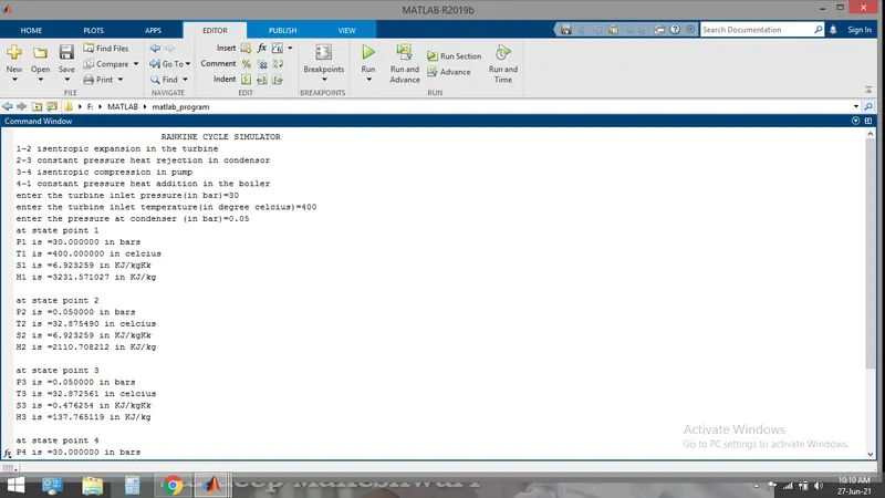
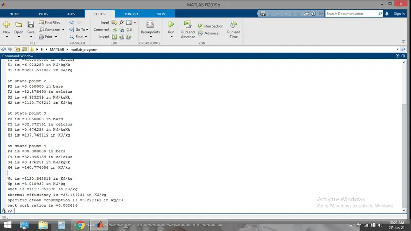
5)the results are displayed in the command window
6)the for loop is used for the plotting of the saturation liquid curve and saturation vapour curve on h-s AND T-s diagram
7)T-s and h-s diagram are plotted using the plot command.
output from the code
image of command window
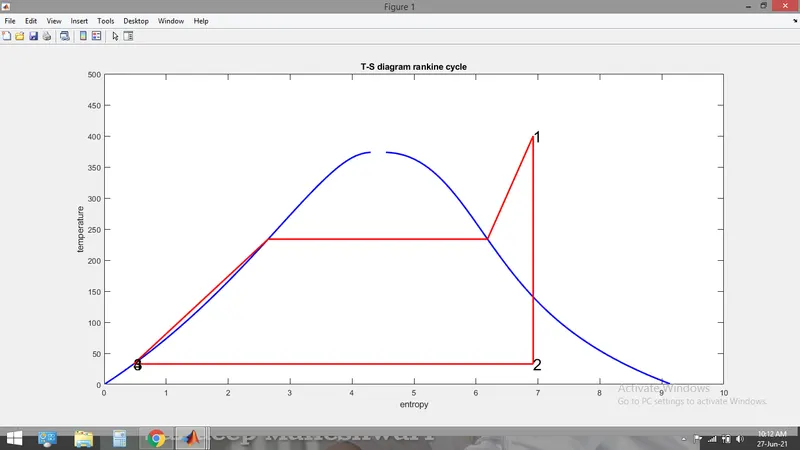
T-S diagram
h-s diagram
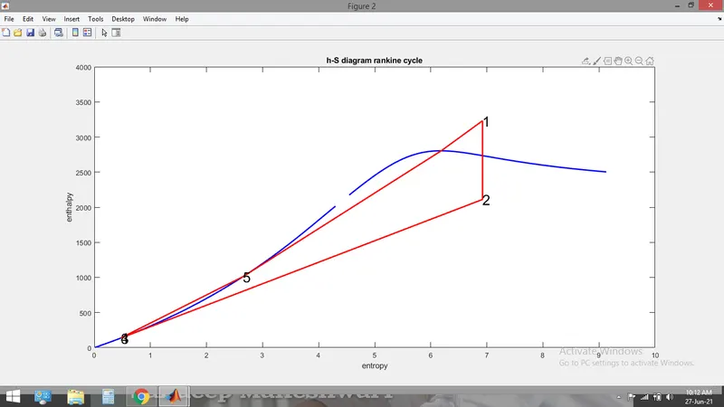
There are discontinuty in the hs and Ts diagram that point is called critical point and properties are not properly defined there in the XSteam library.
The state point 3 and 4 are nearly coincided with each other because the pump work and the temperature difference across the pump is very small.
no major was occurred during the code