Project 2 - Rankine cycle Simulator
OBJECTIVE:
Create a Rankine cycle simulator using MATLAB and evaluating the state points in the cycle provided with required inputs.
PRE-REQUISITES:
i) The steam cycle is a practical cycle and is the basis of virtually all steam power plants and hence electricity generation.
ii) The main difficulties of the Carnot cycle are overcome by complete condensation in the condenser and by superheating which is optional.
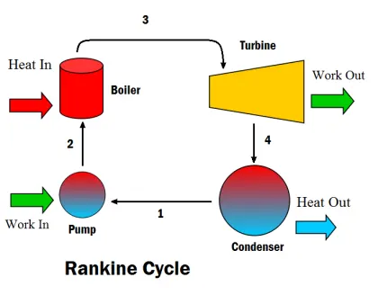
iii) The Rankine cycle includes the following processes:
a) Feed Pump:
The saturated liquid which is the outcome of the condenser enters into the pump which increases its pressure to the boiler pressure isentropically.
b) Boiler:
In the boiler, a constant pressure heat addition process takes place which increases the enthalpy of the working fluid to sufficient value.
c) Turbine:
Isentropic expansion of the working fluid takes place in the turbine which results in work output.
d) Condensor:
In condensor, constant pressure heat rejection process convert all the vapour output of the turbine into saturated liquid.
PROCEDURE:
a) Main Code:
%Rankine Cycle
clear all
close all
clc

disp('                               RANKINE CYCLE                                ');
disp('1-2 is Iscentropic Expansion in the Turbine');
disp('2-3 is Constant Pressure Heat rejection by the Condensor');
disp('3-4 is Iscentropic Expansion in the Pump');
disp('4-1 is Constant Pressure Heat addition to the Boiler');

%Inputs:
disp('                               INPUTS                                  ');
P1 = input('Enter the Pressure at turbine inlet(bar):');
T1 = input('Enter the Temperature at the Turbine inlet(degree C):');
P2 = input('Enter the Pressure at the Condensor(bar):');

%Using the XSteam functions,the enthalpy and entropy at various
%points can be calculated:

%Caluclating enthalpy(h) and entropy(s) at point 1:
h1 = XSteam('h_pT',P1,T1);
s1 = XSteam('s_pT',P1,T1);

%Caluclating pressure(P),enthalpy(h) and entropy(s) at point 2:

%Since Iscentropic Expansion:
s2=s1;

%For Iscentropic Expansion:
% wkt (T2/T1)=(P2/P1)^(1-(1/g))
g = 1.4;
power = 1-(1/g);

%Hence (T2/T1) = (P2/P1)^power:
T2 = T1*((P2/P1)^power);
h2 = XSteam('h_pT',P2,T2);

%Caluclating pressure(P),enthalpy(h) and entropy(s) at point 3:

%Since Constant Pressure Heat Removal:
P3 = P2;
T3 = T2;
h3 = XSteam('hL_T',T3);
s3 = XSteam('sL_T',T3);

%Caluclating pressure(P),enthalpy(h) and entropy(s) at point 4:

%Since Iscentropic Compression:
s4 = s3;

%Since Constant Pressure Process:
P4 = P1;

T4 = XSteam('T_ps',P4,s4);
h4 = XSteam('h_pT',P4,T4);
h41 = XSteam('hL_p',P4);
s41 = XSteam('sL_p',P4);
h42 = XSteam('hV_p',P4);
s42 = XSteam('sV_p',P4);
T41 = XSteam('T_hs',h41,s41);
T42 = XSteam('T_hs',h42,s42);

%Calculating the Entropy and Enthapy at the saturation curve:

Temp = linspace(0,500,600);

for i = 1:length(Temp)

sv(i) = XSteam('sV_T',Temp(i));
sl(i) = XSteam('sL_T',Temp(i));

hv(i) = XSteam('hV_T', Temp(i));
hl(i) = XSteam('hL_T', Temp(i));

end

%Calculating Net Work Output(W_net):

W_t = h1-h2;
W_p = h4-h3;
W_net = W_t-W_p;

%Calculating Back Work Ratio:
Bw_ratio = W_p/W_t;

%Calculating the Thermal efficiency:
Q_in = h1-h4;
eff_thermal = (W_net/Q_in)*100;

%Calculating Specific Steam Consumption:
% wkt 1J = 3600kg/s
SSC = 3600/W_net;

% Displaying Results in the command window:
disp('                       Results                       ');
P1 = P1;
T1 = T1;
P2 = P2;
disp('At stage point 1');
n1 = sprintf('P1 is %.3f bar',P1);
disp(n1);
n2 = sprintf('T1 is %.3f C',T1);
disp(n2);
n3 = sprintf('h1 is %.3f kJ/kg',h1);
disp(n3);
n4 = sprintf('s1 is %.3f kJ/kgK',s1);
disp(n4);
disp('At stage point 2');
n11 = sprintf('P2 is %.3f bar',P2);
disp(n11);
n21 = sprintf('T2 is %.3f C',T2);
disp(n21);
n31 = sprintf('h2 is %.3f kJ/kg',h2);
disp(n31);
n41 = sprintf('s2 is %.3f kJ/kgK',s2);
disp(n41);
disp('At stage point 3');
n12 = sprintf('P3 is %.3f bar',P3);
disp(n12);
n22 = sprintf('T3 is %.3f C',T3);
disp(n22);
n32 = sprintf('h3 is %.3f kJ/kg',h3);
disp(n32);
n42 = sprintf('s3 is %.3f kJ/kgK',s3);
disp(n42);
disp('At stage point 4');
n13 = sprintf('P4 is %.3f bar',P4);
disp(n13);
n23 = sprintf('T4 is %.3f C',T4);
disp(n23);
n33 = sprintf('h4 is %.3f kJ/kg',h4);
disp(n33);
n43 = sprintf('s4 is %.3f kJ/kgK',s4);
disp(n43);
n14 = sprintf('W_t is %.3f kJ/kg',W_t);
disp(n14);
n15 = sprintf('W_p is %.3f kJ/kg',W_p);
disp(n15);
n16 = sprintf('W_net is %.3f kJ/kg',W_net);
disp(n16);
n17 = sprintf('Eff_Thermal is %.2f Percent',eff_thermal);
disp(n17);
n18 = sprintf('SSC is %.2f kg/kWh',SSC);
disp(n18);

figure(1)
plot([s1 s2],[T1 T2],[s2 s3],[T2 T3],[s3 s4],[T3 T4],[s4 s41],[T4 T41],[s41 s42],[T41 T42],[s42 s1],[T42 T1],'marker','*','color','r')
hold on
plot(sv,Temp)
plot(sl,Temp)
xlabel('Entropy-s(kJ/kgK');
ylabel('Temperature-T(K)');

figure(2)
plot([s1 s2],[h1 h2],[s2 s3],[h2 h3],[s3 s4],[h3 h4],[s4 s1],[h4 h1],'marker','*','color','g')
hold on
plot(sv,hv)
plot(sl,hl)
xlabel('Entropy-s(kJ/kgK');
ylabel('Enthalpy-h(kJ/k)');
b) Steps involved:
i) Option to provide input values is provided using inputdlg command with default input values.
ii) Since the values received are string, they are converted into numeric values using str2num command.
iii) Parameters at different states are evaluated using XSteam function with the help of input parameters.
iv) At state 3, which is the turbine inlet, there are three possibilities.
v) The first is provided temperature at the turbine inlet is less than saturation temperature at the provided boiler pressure.
vi) In this case, data is impractical and no calculation of the other states can be made.
vii) The other two cases are that the turbine inlet condition is equal to vapour saturation temperature or the working fluid is superheated.
viii) These condition at state 3 is provided using if-else-if command.
ix) Once the thermodynamic parameters at all states are known, net work done and back work ratio is evaluated.
x) Output is printed using fprintf command.
xi) To plot the curve, it is necessary to know the extreme limits of the pressure which is possible.
xii) Along with that pressure limits, saturation temperature, saturation liquid entropy and saturation vapour enthalpy are evaluated.
xiii) To know the pressure lower limits while loop is used with a condition that pressure value keeps decreasing till it ceases to exist.
xiv) For this purpose, isnan command is used.
xv) Similarly, for pressure upper limits, pressure is increased till it ceases to exist.
xvi) Once the pressure limit is known saturation temperature, saturation liquid entropy and saturation vapour enthalpy are evaluated and using the plot command, the results are plotted.
xvii) The Rankine cycle states are also plotted in the same figure using hold on command including the possible variation at state 3.
xviii) Legend, title, axis labels and text are added to the plot for clear representation.
xix) To plot the H-S diagram, enthalpy values are evaluated between extreme limits of pressure.
xx) The graph is plotted and labelled in the same way as for the T-S diagram.
RESULTS:
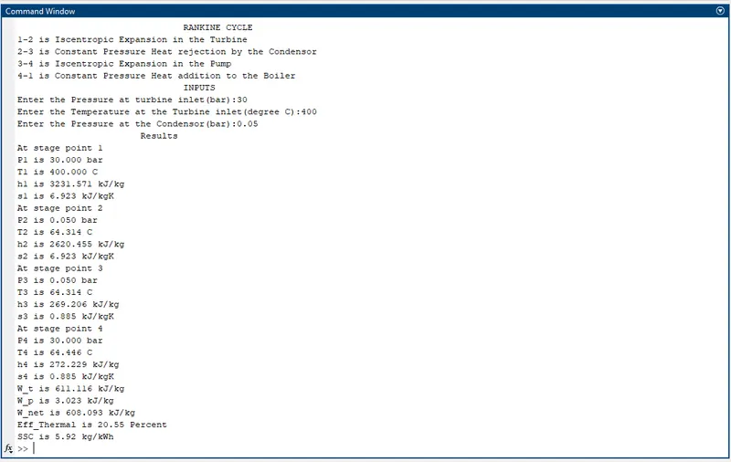
i) The following output was obtained:
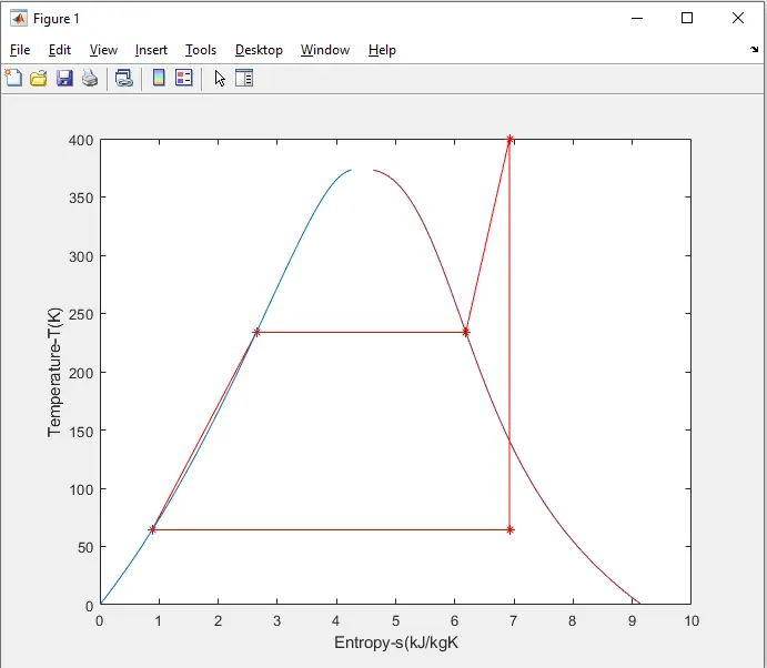
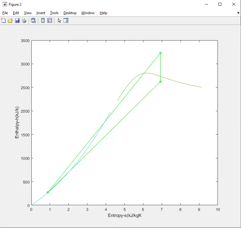
ii) The T-S and H-S plots are displayed below:
CONCLUSION:
i) All the state points of the Rankine cycle is calculated depending upon the provided inputs with the option of superheating at the turbine inlet.
ii) The T-S and H-S diagram is plotted based on the results obtained.