Rankine cycle

The Rankine cycle is a model used to predict the performance of steam turbine systems. It was also used to study the performance of reciprocating steam engines. The Rankine cycle is an idealized thermodynamic cycle of a heat engine that converts heat into mechanical work while undergoing phase change.

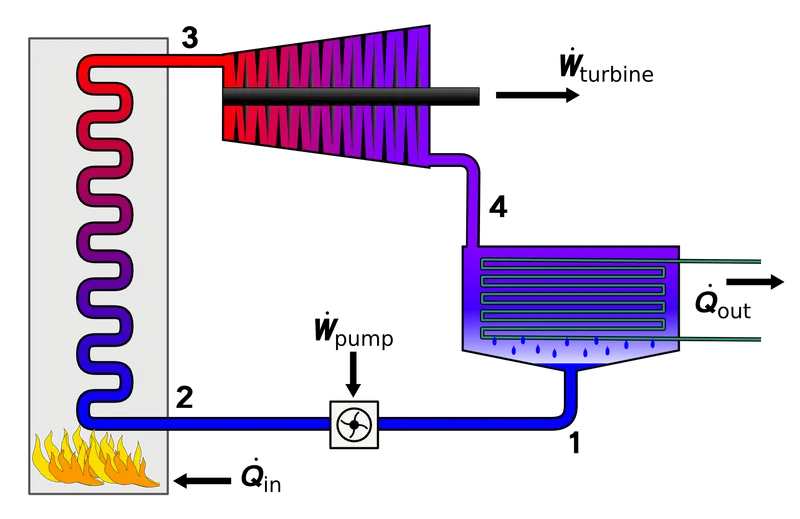
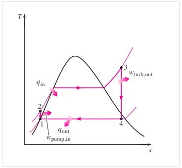
Water enters the pump at state 1 as saturated liquid and is compressed isentropically to the operating pressure of the boiler. The water temperature increases somewhat during this isentropic compression process due to a slight decrease in the specific volume of water. The vertical distance between states 1 and 2 on the T-s diagram is greatly exaggerated for clarity. Water enters the boiler as a compressed liquid at state 2 and leaves as a superheated vapor at state 3. The boiler is basically a large heat exchanger where the heat originating from combustion gases, nuclear reactors, or other
sources is transferred to the water essentially at constant pressure. The boiler, together with the section where the steam is superheated (the superheater), is often called the steam generator.
The superheated vapor at state 3 enters the turbine, where it expands isentropically and produces work by rotating the shaft connected to an electric generator. The pressure and the temperature of steam drop during this process to the values at state 4, where steam enters the condenser. At this state, steam is usually a saturated liquid–vapor mixture with a high quality. Steam is condensed at constant pressure in the condenser, which is basically a large heat
exchanger, by rejecting heat to a cooling medium such as a lake, a river, or the atmosphere. Steam leaves the condenser as saturated liquid and enters the pump, completing the cycle. In areas where water is precious,
the power plants are cooled by air instead of water. This method of cooling, which is also used in car engines, is called dry cooling. Several power plants in the world, including some in the United States, use dry cooling to conserve water.
Remembering that the area under the process curve on a T-s diagram represents the heat transfer for internally reversible processes, we see that the area under process curve 2-3 represents the heat transferred to the
water in the boiler and the area under the process curve 4-1 represents the heat rejected in the condenser. The difference between these two is the net work produced during the cycle.

The four processes in the Rankine cycle

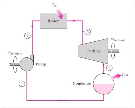
There are four processes in the Rankine cycle. The states are identified by numbers (in brown) in the T-s diagram.

• Process 1–2: The working fluid is pumped from low to high pressure. As the fluid is a liquid at this stage, the pump requires little input energy.

In other words Process 1-2 is [Isentropic compression]

• Process 2–3: The high-pressure liquid enters a boiler, where it is heated at constant pressure by an external heat source to become a dry saturated vapour. The input energy required can be easily calculated graphically, using an enthalpy–entropy chart (h–s chart, or Mollier diagram), or numerically, using steam tables.

In other words Process 2-3 is [Constant pressure heat addition in boiler]

• Process 3–4: The dry saturated vapour expands through a turbine, generating power. This decreases the temperature and pressure of the vapour, and some condensation may occur. The output in this process can be easily calculated using the chart or tables noted above.

In other words Process 3-4 is [Isentropic expansion]

• Process 4–1: The wet vapour then enters a condenser, where it is condensed at a constant pressure to become a saturated liquid.

In other words Process 4-1 is [Constant pressure heat rejection in condenser]

T-s diagram

CODE

clear all
close all
clc
% displaying rankine cycle simulator and its processess
disp("         Rankine cycle simulator")
fprintf(' 1-2  is the  isentropic expansion process');fprintf('.n');
fprintf(' 2-3  is the constant pressure heat rejection process');fprintf('.n');
fprintf(' 3-4  is the isentropic compression process');fprintf('.n');
fprintf(' 4-1  is the constant pressure heat addition process');fprintf('.n');
fprintf('   n');
% Inputs
p1 = 30;
t1 = 400;
p2 =0.05;


% variables for stage 1
p1 = 30;
t1 = 400;
h1=XSteam('h_pT',p1,t1);
s1=XSteam('s_pT',p1,t1);
fprintf('          Result');fprintf('sn');
fprintf('   n');
fprintf('    At state point 1');fprintf('.n');
fprintf(' P1 is:%f bar',p1);fprintf('.n');
fprintf(' T1 is:%f deg celcius',t1);fprintf('.n');
fprintf(' H1 is:%f KJ/Kg',h1);fprintf('.n');
fprintf(' S1 is:%f KJ/KgK',s1);fprintf('.n');
fprintf('   n');

% variables for stage 2
p2 =0.05;
s2=s1;
t2=XSteam('T_ps',p2,s2);
sf2 = XSteam('sL_p',p2);
sg2 = XSteam('sV_p',p2);
hf2 = XSteam('hL_p',p2);
hg2 = XSteam('hV_p',p2);
x = ((s2 - sf2)/(sg2 - sf2));
h2 = hf2 + (x*(hg2 - hf2));
fprintf('    At state point 2');fprintf('.n');
fprintf(' P2 is:%f bar',p2);fprintf('.n');
fprintf(' T2 is:%f deg celcius',t2);fprintf('.n');
fprintf(' H2 is:%f KJ/Kg',h2);fprintf('.n');
fprintf(' S2 is:%f KJ/KgK',s2);fprintf('.n');
fprintf('   n');



% variables for stage 3
p3=p2;
t3=t2;
h3=XSteam('hL_T',t3);
s3=XSteam('sL_p',p3);
fprintf('    At state point 3');fprintf('.n');
fprintf(' P3 is:%f bar',p3);fprintf('.n');
fprintf(' T3 is:%f deg celcius',t3);fprintf('.n');
fprintf(' H3 is:%f KJ/Kg',h3);fprintf('.n');
fprintf(' S3 is:%f KJ/KgK',s3);fprintf('.n');
fprintf('   n');


% variables for stage 4
p4=p1;
s4=s3;


t4=t3*((p4/p3)^0);

v3=XSteam('vL_p',p3);
Wp=v3*((p4-p3)*100);
h4=h3+Wp;
fprintf('    At state point 4');fprintf('.n');
fprintf(' P4 is:%f bar',p4);fprintf('.n');
fprintf(' T4 is:%f deg celcius',t4);fprintf('.n');
fprintf(' H4 is:%f KJ/Kg',h4);fprintf('.n');
fprintf(' S4 is:%f KJ/KgK',s4);fprintf('.n');
fprintf('   n');

% variables for stage 5
p5=p1;
t5=XSteam('Tsat_p',p5);
s5=XSteam('sL_p',p5);
h5=XSteam('hL_T',t5);
fprintf('    At state point 5');fprintf('.n');
fprintf(' P5 is:%f bar',p5);fprintf('.n');
fprintf(' T5 is:%f deg celcius',t5);fprintf('.n');
fprintf(' H5 is:%f KJ/Kg',h5);fprintf('.n');
fprintf(' S5 is:%f KJ/KgK',s5);fprintf('.n');
fprintf('   n');

% variables for stage 6
t6=t5;
p6=XSteam('psat_T',t5);
s6=XSteam('sV_T',t6);
h6=XSteam('hV_T',t6);
fprintf('    At state point 6');fprintf('.n');
fprintf(' P6 is:%f bar',p6);fprintf('.n');
fprintf(' T6 is:%f deg celcius',t6);fprintf('.n');
fprintf(' H6 is:%f KJ/Kg',h6);fprintf('.n');
fprintf(' S6 is:%f KJ/KgK',s6);fprintf('.n');
fprintf('   n');


% Pump work
Wp=v3*((p4-p3)*100);
fprintf(' Wp is:%f KJ/Kg',Wp);fprintf('.n');
% Turbine work
Wt=h1-h2;
fprintf(' Wt is:%f KJ/Kg',Wt);fprintf('.n');
% Net work
Wnet=Wt-Wp;
fprintf(' Wnet is:%f KJ/Kg',Wnet);fprintf('.n');
% Heat in
Qin=h1-h4;
% Heat out
Qout=h2-h3;
% Thermodynamic efficiency
Ntherm=Wnet/Qin;
fprintf(' Ntherm is:%f KJ/Kg',Ntherm);fprintf('.n');
% Specific steam consumption
ssc = 3600/Wnet;
fprintf(' S.S.C is:%f KJ/Kg',ssc);fprintf('.n');


t = linspace(0,400,1000);
for i=1:length(t)
s_line1(i)=XSteam('sL_T',t(i));
end

for j=1:length(t)
s_line2(j)=XSteam('sV_T',t(j));
end
for i=1:length(t)
h_line1(i)=XSteam('hL_T',t(i));
end

for j=1:length(t)
h_line2(j)=XSteam('hV_T',t(j));
end


%plotting s-t graph
figure(1)
hold on
plot([s_line1 s_line2],[t t],'linewidth',2,'color','r')
plot([s1 s2 s3 s4 s5 s6 s1],[t1 t2 t3 t4 t5 t6 t1],'linewidth',2,'color','black')
text(s1,t1,'1')
text(s2,t2,'2')
text(s3,t3,'3')
text(s4,t4,'4')
text(s5,t5,'5')
text(s6,t6,'6')
title("Rankine cycle T-S Diagram")
xlabel('Entropy(KJ/KgK)')
ylabel('Temperature(K)')

%plotting h-s graph
figure(2)
hold on
plot([s_line1 s_line2],[h_line1 h_line2],'linewidth',2,'color','r')
plot([s1 s2 s3 s4 s5 s6 s1],[h1 h2 h3 h4 h5 h6 h1],'linewidth',2,'color','black')
text(s1,h1,'1')
text(s2,h2,'2')
text(s3,h3,'3')
text(s4,h4,'4')
text(s5,h5,'5')
text(s6,h6,'6')
title("Rankine cycle H-S Diagram")
xlabel('Entropy(KJ/KgK)')
ylabel('Enthalpy(KJ/Kg)')

CODE EXPLANATION

• Starting with clear all, close all and clc
• Inputs p1 = 30 bars
  t1 = 400 degree celsius
  p2 =0.05 bars
• Finding the variables stage by stage

@stage 1

• At Turbine inlet temperature and pressure are given

  Turbine Inlet temperature = 400° C

  Turbine Inlet Pressure = 30 bars

• And we have to find out the entropy(S) and enthalpy(H)

• Click here to download the Xsteam Library. We i'll be calling the funtion from this steam data file as shown

• h1=XSteam('h_pT',p1,t1)
  s1=XSteam('s_pT',p1,t1)

@stage 2

• At Turbine outlet Pressure = 0.05 bars = Condenser Inlet Pressure
• Rest of variables are find using file as shown
• temperature t2=XSteam('T_ps',p2,s2)
• sf2 = XSteam('sL_p',p2)
  sg2 = XSteam('sV_p',p2)
  hf2 = XSteam('hL_p',p2)
  hg2 = XSteam('hV_p',p2)
  x = ((s2 - sf2)/(sg2 - sf2))
  h2 = hf2 + (x*(hg2 - hf2))
• x is the length from the point 2 to 3 and by using that we ill be finding the enthalpy as shown above
• And entropy s2 = s1

@stage 3

• Pressure p3=p2
  temperature t3=t2
• enthalpy h3=XSteam('hL_T',t3)
  entropy s3=XSteam('sL_p',p3)

@stage 4

• Pressure p4=p1
  entropy s4=s3
• temperature t4=t3*((p4/p3)^0)
• enthalpy v3=XSteam('vL_p',p3)
  pump work Wp=v3*((p4-p3)*100)
  h4=h3+Wp
• For the enthalpy h4 = enthalpy at stage 3 + pump work

@stage 5

• Pressure p5=p1
  temperature t5=XSteam('Tsat_p',p5)
  entropy s5=XSteam('sL_p',p5)
  enthalpy h5=XSteam('hL_T',t5)

@stage 6

• temperature t6=t5
  Pressure p6=XSteam('psat_T',t5)
  entropy s6=XSteam('sV_T',t6)
  enthalpy h6=XSteam('hV_T',t6)

Pump work
Wp=v3*((p4-p3)*100)

Turbine work
Wt=h1-h2

Net work
Wnet=Wt-Wp

Heat in
Qin=h1-h4

Heat out
Qout=h2-h3

Thermodynamic efficiency
Ntherm=Wnet/Qin

Specific steam consumption
ssc = 3600/Wnet

The specific steam consumption is defined as the steam consumed by one cylinder of locomotives per unit of power. Normally, it is measured in kgkWh or kgKJ. Specific steam consumption is the amount of steam a locomotive's cylinders consume. It can be measured in kWh or KJ.

• And for the saturated liquid and vapour lline we i'll be doing as shown

t = linspace(0,400,1000);
for i=1:length(t)
s_line1(i)=XSteam('sL_T',t(i));
end

for j=1:length(t)
s_line2(j)=XSteam('sV_T',t(j));
end
for i=1:length(t)
h_line1(i)=XSteam('hL_T',t(i));
end

for j=1:length(t)
h_line2(j)=XSteam('hV_T',t(j));
end

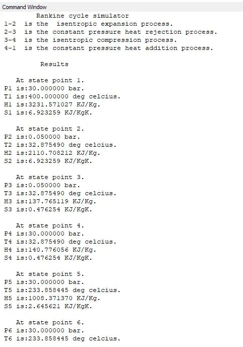
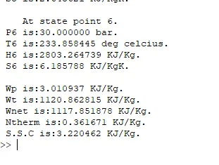
RESULTS

PLOTS

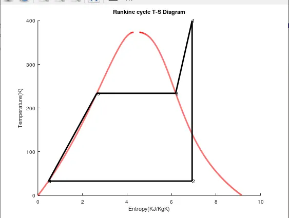
T-S Diagram

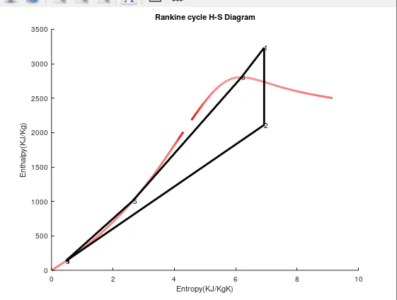
H-S Diagram

COMMAND WINDOW