Rankine cycle Simulator using MATLAB
Aim – To develop a code to solve the rankine cycle problem and plot the Pressure-Enthalpy diagram and Enthalpy-Entropy diagram of a rankine cycle.
Introduction – Rankine cycle is commonly used cycle for converting the heat energy from boiler to mechanical energy using turbine and then it is further stored in the form of electrical energy.
Rankine cycle consists of following four processes.
Process 1-2: Isentropic Expansion
Process 2-3: Constant Pressure Heat Rejection
Process 3-4: Isentropic Compression by the Pump
Process 4-1: Constant Pressure Heat Addition
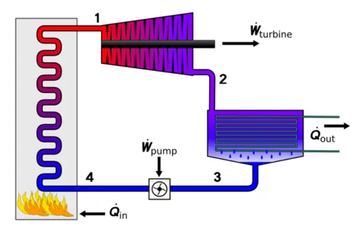
Description of this processes is as follows.
Process 3-4: Pump pumps the water from low pressure to high pressure. The water enters into pump at saturated liquid state. The liquid is compressed isentropically till the boiler pressure. Work required for the pump is given as:
Wpump = m(h3 – h4) kW
Process 4-1: With the help of external fuel, water is converted into superheated steam in the boiler. The phase is change during this process. Heat supplied to the boiler is given as:
Qsupplied = m(h1 – h4) kW
Proess 1-2: Superheated steam from boiler enters into the turbine, which expands in the turbine isentropically and mechanical work is produced. Later, generator converts this mechanical work into electrical energy.
Work generated by the turbine is given as,
Wturbine = m(h1 – h2) kW
Process 2-3: Condenser lowers the temperature of steam and condenses into liquid. Phase is changed from vapour to liquid state during condensation process and this condensed liquid is again supplied to the pump.
Heat rejected in the condenser is given as:
Qrejected = m(h2 – h3) kW
Code to solve the rankine cycle and to generate T-S and H-S diagram
clear all
close all
clc

%Display Screen
disp('Rankine Cycle');
disp('1-2: Isentrpic Expansion in the Turbine');
disp('2-3: Constant Pressure Heat rejection by the Pump');
disp('3-4: Isentropic Compression by the Pump');
disp('4-1: Constant Pressure heat addition by the boiler');

%Inputs
p1 = input('Enter the Pressure at the turbine inlet in Bar : ');
t1 = input('Enter the temperature at the turbine inlet in deg C : ');
p3 = input('Enter the pressure at the condenser in Bar : ');

%Calculations
p4 = p1;
p2 = p3;
%Point 3
h3 = XSteam('hL_p',p3);
s3 = XSteam('sL_p',p3);
t3 = XSteam('Tsat_p',p3);
v3 = XSteam('vL_p',p3);

s1 = XSteam('s_pT',p1,t1);
h1 = XSteam('h_pT',p1,t1);

%Point 2
s2 = s1;
t2 = t3;
sf2 = XSteam('sL_p',p2);
sg2 = XSteam('sV_p',p2);
hf2 = XSteam('hL_p',p2);
hg2 = XSteam('hV_p',p2);
x2 = ((s2-sf2)/(sg2-sf2));
h2 = hf2 + x2*(hg2-hf2);

%Point 4
s4 = s3;
pump_work = v3*(p4-p3)*100;
h4 = h3 + pump_work;

cp4 = XSteam('Cp_ps',p4,s4);
cv4 = XSteam('Cv_ps',p4,s4);
gamma = cp4/cv4;

t4 = t3*(p4/p3)^((gamma-1)/gamma);

%Point 5
p5 = p1;
t5 = XSteam('Tsat_p',p5);
s5 = XSteam('sL_p',p5);
h5 = XSteam('hL_p',p5);

%Point 6
p6 = p1;
t6 = XSteam('Tsat_p',p6);
s6 = XSteam('sV_p',p6);
h6 = XSteam('hV_p',p6);

%Net Work
Wturbine = h1 - h2;
Wpump = h4 - h3;
Wnet = Wturbine - Wpump;

%Back Work Ratio
BWR = Wpump/Wturbine;

%%Heat supplied in Boiler
qboiler = h1 - h4;

%Efficiency of a rankine cycle
Eff = (Wnet/qboiler)*100;

%Specific Steam Consumption
m = 1;
Sfc = (m*Wnet)/3600;
%Finding the curve from point 6 to 1

t6_1 = linspace(t6,t1,1000);

for i = 1:length(t6_1)
    s6_1(i) = XSteam('s_pT',p6,t6_1(i));
    h6_1(i) = XSteam('h_pT',p6,t6_1(i));
end

%Finding the values of Enthalpy and Entropy in Saturation Curve
t_total = linspace(0,t1,1000);

for i = 1:length(t_total)
    h_total(i) = XSteam('hL_T',t_total(i));
    s_total(i) = XSteam('sL_T',t_total(i));
    H_total(i) = XSteam('hV_T',t_total(i));
    S_total(i) = XSteam('sV_T',t_total(i));
end

%Plotting
figure(1)
plot(s_total,t_total)
hold on
plot(S_total,t_total)
hold on
plot(s6_1,t6_1)
hold on
plot([s1 s2],[t1 t2])
hold on
plot([s2 s3],[t2 t3])
hold on
plot([s3 s4],[t3 t4])
hold on
plot([s4 s5],[t4 t5])
hold on
plot([s5 s6],[t5 t6])
xlabel('Entropy [kJ/kgK]')
ylabel('Temperature [Deg C]')
title('Entropy vs Temperature')

figure(2)
plot(s_total,h_total)
hold on
plot(S_total,H_total)
hold on
plot([s1 s2],[h1 h2])
hold on
plot([s2 s3],[h2 h3])
hold on
plot([s3 s4],[h3 h4])
hold on
plot([s4 s5],[h4 h5])
hold on
plot([s5 s6],[h5 h6])
hold on
plot(s6_1,h6_1)
xlabel('Entropy [kJ/kgK]')
ylabel('Enthalpy [kJ/kg]')
title('Entropy vs Enthalpy')

%Results
fprintf('nResults');
fprintf('nAt State Point 1');
fprintf('nP1 is : %4.2f Bar',p1);
fprintf('nT1 is : %4.2f Deg Celcius',t1);
fprintf('nH1 is : %4.2f kJ/kg',h1);
fprintf('nS1 is : %4.2f kJ/kgKn',s1);

fprintf('nAt State Point 2');
fprintf('nP2 is : %4.2f Bar',p2);
fprintf('nT2 is : %4.2f Deg Celcius',t2);
fprintf('nH2 is : %4.2f kJ/kg',h2);
fprintf('nS2 is : %4.2f kJ/kgKn',s2);

fprintf('nAt State Point 3');
fprintf('nP3 is : %4.2f Bar',p3);
fprintf('nT3 is : %4.2f Deg Celcius',t3);
fprintf('nH3 is : %4.2f kJ/kg',h3);
fprintf('nS3 is : %4.2f kJ/kgKn',s3);


fprintf('nAt State Point 4');
fprintf('nP4 is : %4.2f Bar',p4);
fprintf('nT4 is : %4.2f Deg Celcius',t4);
fprintf('nH4 is : %4.2f kJ/kg',h4);
fprintf('nS4 is : %4.2f kJ/kgKn',s4);

fprintf('nWork done by Turbine is : %4.2f kJ/kg', Wturbine);
fprintf('nWork required by pump is : %4.2f kJ/kg', Wpump);
fprintf('nNet Work is : %4.2f kJ/kg', Wnet);
fprintf('nThermal Efficiency is : %4.2f Percent', Eff);
fprintf('nBack Work Ratio is : %4.4f', BWR);
fprintf('nSpecific Steam Consmption is : %4.2f Kg/Kwh', Sfc);
Explanation of the Code –
XSteam is the file saved in the same directory of the program from which all the values of various states are taken.
First, inputs are given as pressure and temperature of steam entering in the turbine and pressure of the condenser by the input command. Pressure at state 1 is equal to pressure at state 4 and pressure at state 2 is equal to pressure at state 3. After equating this, state values of enthalpy, entropy and temperature at point 3 (saturation point) are found out. At point 1, enthalpy and entropy are found out using the inputs.
Entropy at point 1 and 2 is constant due to isentropic process and temperature at point 2 and 3 is same. Then dryness fraction and enthalpy at point 2 is found out by solving the equations. Similarly at point 4, the enthalpy is calculated from pump work, temperature at point 4 is calculated from adiabatic index and air standard cycle equation. Consequently, the values of states at point 5 and 6 are calculated.
Net work is calculated as the difference of turbine work and the pump work. Ratio of net work to the heat supplied gives the efficiency of the cycle. Similarly, by assuming mass flow is equal to 1kg/sec, specific steam consumption is found out as a multiplication of net work and mass flow in kg/kWh.
To calculate the curve from point 6 to point 1 in T-S diagram, all the values of temperature are taken from t6 to t1 with 1000 parts between them and similarly using for loop h and s values between this points are found out. Maximum temperature in the diagram is at t1. Hence, in order to plot the saturation curve, temperature values from 0 to t1 with 1000 parts are taken as a function of linspace command and h and s values at vapour and liquid states are found out using for loop.
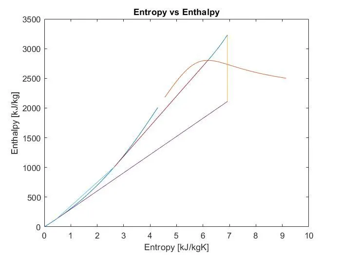
All the values from point 1 to 6 are plotted and values of saturation curve are also plotted to create two figures (i.e. T-S and H-S plots). The calculation results is displayed using fprintf command and n displays the result on the next line in command window. %f is used to display floating variable and 4.2 is the variables description (i.e. for 2 decimal values and 4 places should be free). Result of plots and calculations are shown below.
Results –
Inputs for the problem are taken as,
- Turbine Inlet Temperature – 400 Deg C
- Turbine Inlet Pressure – 30 Bar
- Turbine Outlet Pressure= Condenser Pressure – 0.05 Bar
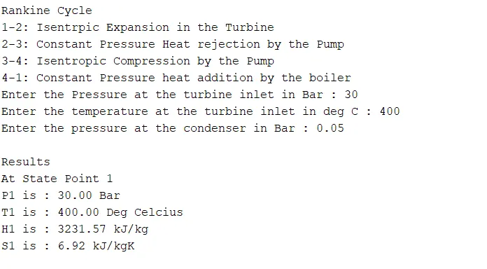
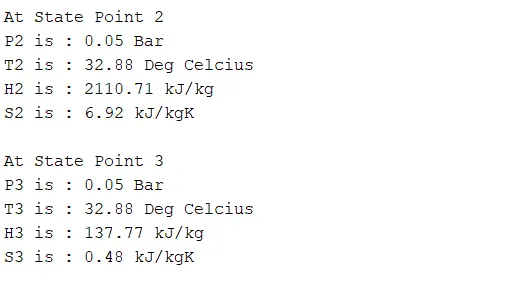
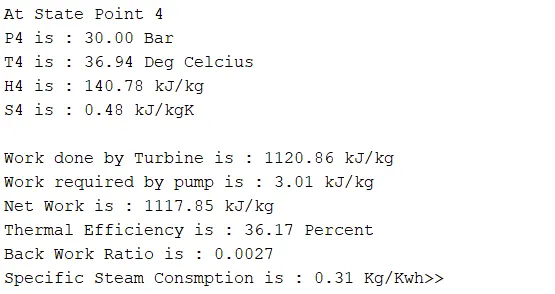
Plots of H-S and T-S diagram-
- Temperature- Entropy (T-S) Diagram
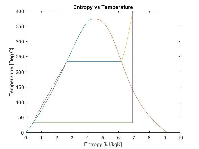
Note: The plot of temperature and entropy between point 3 and point 4 is very short due to very less condensation pressure (i.e. 0.05 Bar). Hence, isentropic compression process 3-4 can only be seen by zooming the points.
2. Enthalpy- Entropy (H-S) Diagram –