Creating a Rankine cycle Simulator using MATLAB.
Project2 Report.
- Aim: To write a code that calculates the properties at all the state points and then plots the Temperature-Entropy and the Enthalpy-Entropy Diagram for the given Rankine Cycle.
- Introduction:
The Rankine cycle is a model used to predict the performance of steam turbine systems. It was also used to study the performance of reciprocating steam engines. The Rankine cycle is an idealized thermodynamic cycle of a heat engine that converts heat into mechanical work while undergoing phase change. It is an idealized cycle in which friction losses in each of the four components are neglected. The heat is supplied externally to a closed loop, which usually uses water as the working fluid. It is named after William John Macquorn Rankine, a Scottish polymath and Glasgow University professor.
The Rankine cycle closely describes the process by which steam-operated heat engines commonly found in thermal power generation plants generate power.
Power depends on the temperature difference between a heat source and a cold source. The higher the difference, the more mechanical power can be efficiently extracted out of heat energy, as per Carnot's theorem.
The Heat sources used in these power plants are usually nuclear fission or the combustion of fossil fuels such as coal, natural gas, and oil, or concentrated solar power. The higher the temperature, the better.
The efficiency of the Rankine cycle is limited by the high heat of vaporization of the working fluid. Also, unless the pressure and temperature reach super critical levels in the steam boiler, the temperature range the cycle can operate over is quite small: steam turbine entry temperatures are typically around 565 °C and steam condenser temperatures are around 30 °C. This gives a theoretical maximum Carnot efficiency for the steam turbine alone of about 63.8% compared with an actual overall thermal efficiency of up to 42% for a modern coal-fired power station. This low steam turbine entry temperature (compared to a gas turbine) is why the Rankine (steam) cycle is often used as a bottoming cycle to recover otherwise rejected heat in combined-cycle gas turbine power stations.
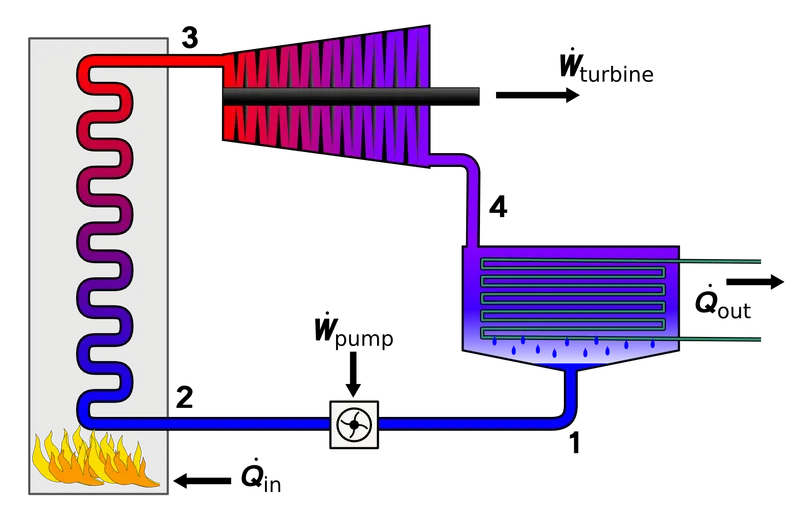
Typical Rankine Cycle Layout.
Here:
1:Pump
2: Boiler
3: Turbine
4: Condenser
A typical TS diagram will look something like the following: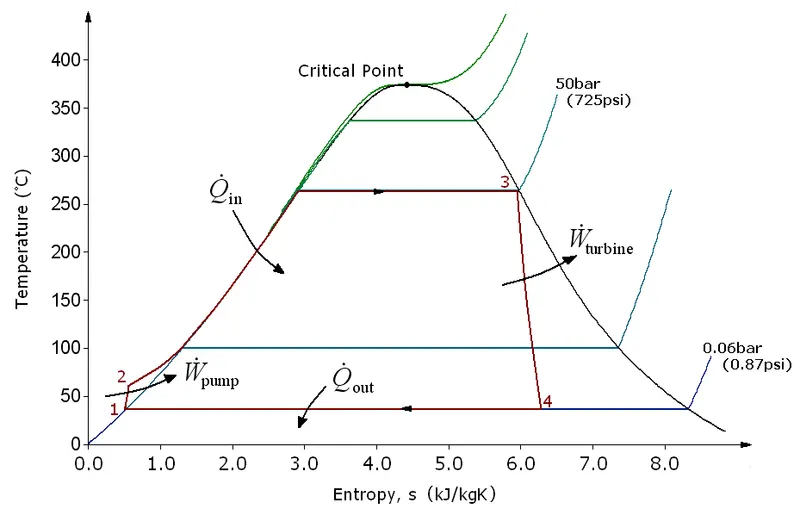
TS diagram of the Rankine Cycle
There are four processes in the Rankine cycle. The states are identified by numbers (in brown) in the T–s diagram.- Process 1–2: The working fluid is pumped from low to high pressure. As the fluid is a liquid at this stage, the pump requires little input energy.
In other words Process 1-2 is [Isentropic compression]
- Process 2–3: The high-pressure liquid enters a boiler, where it is heated at constant pressure by an external heat source to become a dry saturated vapour. The input energy required can be easily calculated graphically, using an enthalpy–entropy chart (h–s chart, or Mollier diagram), or numerically, using steam tables.
In other words Process 2-3 is [Constant pressure heat addition in boiler]
- Process 3–4: The dry saturated vapour expands through a turbine, generating power. This decreases the temperature and pressure of the vapour, and some condensation may occur. The output in this process can be easily calculated using the chart or tables noted above.
In other words Process 3-4 is [Isentropic expansion]
- Process 4–1: The wet vapour then enters a condenser, where it is condensed at a constant pressure to become a saturated liquid.
In other words Process 4-1 is [Constant pressure heat rejection in condenser]
Equations:
In an ideal Rankine cycle the pump and turbine would be isentropic, i.e., the pump and turbine would generate no entropy and hence maximize the net work output. Processes 1–2 and 3–4 would be represented by vertical lines on the T–s diagram and more closely resemble that of the Carnot cycle. The Rankine cycle shown here prevents the state of the working fluid from ending up in the superheated vapor region after the expansion in the turbine, which reduces the energy removed by the condensers.
In general, the efficiency of a simple rankine cycle can be written as

Each of the next four equations is derived from the energy and mass balance for a control volume.
 defines the thermodynamic efficiency of the cycle as the ratio of net power output to heat input. As the work required by the pump is often around 1% of the turbine work output, it can be simplified.
When dealing with the efficiencies of the turbines and pumps, an adjustment to the work terms must be made:
A typical HS Diagram will look something like the following:
Entropy-Enthalpy Diagram - Code/Logic:
1. We firstly need to clear and close all the previously entered codes and the present values of the already used variables, hence we use the following commands:
clear all
close all
clc
2. We begin this code by printing the Introduction and introducing the cycle. For this, we can use the sprintf command. This command will print the string and then store it in a variable. We then display this variable as the output.
str = sprintf(formatSpec,A1,...,An) [str,errmsg] = sprintf(formatSpec,A1,...,An) str = sprintf(literalText)
3. After Introducing the Cycle, we then give the general inputs. The Pressure and Temperatures at state point 1 are mentioned as p1 and t1. The Pressure at state point2 is mentioned as p2.
The values are :
p1 = 30 bar
t1 = 400K
p2 = 0.05 bar
4. After this, we then proceed to calculate the values of Pressure, Temperature and Entropy at the four State points.
So, the Temperature at state points 2,3,4 will be under the variable of t2, t3, t4. And just like this, we can name all the neccessary variables and calculate them accordingly.
Here, we also use the Steam Table that is present in MATLAB. This table gives us the values of Entropy, Enthalpy, and many other thermodynamic properties as a function of Pressure, Temperature etc. We can get the Values of Enthalpy and Entropy of the liquid at Saturated vapour phase as well.
For example: When we use h3 = XSteam('hV_T', t1); this calculates Saturated vapour enthalpy as a function of t1 and assigns the numerical value to the variable of h3.
So, using the appropriate formulae, we then calculate the state points and the various thermodynamic properties as well.
5. After we calculate the basic thermodynamic properties, we then go on to calculate the efficiency of the entire cycle.
5.1 The efficiency is given by:Ntherm = (Wnet /Qin)*100
Here:
Wnet = Net-work done by the cycle.
Qin = Heat input to the cycle.
5.2 The Back Work Ratio is given by:
`"Bwork" = (wp) / (Wt)`
where:
wp = Work done by the Pump.
Wt = Work done by the Turbine.
5.3 Net-Work Done is given by:
`"Nwork" = (Wt-wp) / (Wt)`
where:
wp = Work done by the Pump.
Wt = Work done by the Turbine.
6. Now, after all the calculations are done, we can proceed to plot the graphs and then display the results that we have gotten. To do this, we can use a for loop and then make the loop run between 1 to 4 as there are 4 state points.
So, I have created a variable that will define what it is that is to be printed. And then I put this variable to display. This command will run for all the four iterations and display all the variables. This operation basically condenses the code and makes it much more optimised.
The methodology is shown in the main code below.
7. To plot the graphs, we have used the plot command. The Syntax for that command is shown below:
plot(X,Y) plot(X,Y,LineSpec) plot(X1,Y1,...,Xn,Yn) plot(X1,Y1,LineSpec1,...,Xn,Yn,LineSpecn) plot(Y) plot(Y,LineSpec) plot(___,Name,Value) plot(ax,___) h = plot(___)
All these syntax can be used as per their own use and need.
So, to plot the Saturation Curve in the Temperature-Entropy Plot, we need to calculate the Entropy and Enthalpy at Saturated Vapour and Liquid phases of the working fluid, which in our case is water.
We plot the TS diagram in a seperate figure window and the HS diagram in a seperate figure window.
The code for both of them are given below.We have also used the text command to print the State point numbers at the points.
The syntax for this command is:
text(x,y,txt) text(x,y,z,txt) text(___,Name,Value) text(ax,___) t = text(___)
Main Code:
clear all close all clc %Introduction a = sprintf("RANKINE CYCLE SIMULATOR"); disp(a) b = sprintf(" 1-2 ISENTROPIC EXPANSION IN TURBINE"); disp(b) c = sprintf(" 2-3 CONSTANT PRESSURE HEAT REJECTION BY CONDENSER"); disp(c) d = sprintf(" 3-4 ISENTROPIC COMPRESSION IN PUMP"); disp(d) e = sprintf(" 4-1 CONSTANT PRESSURE HEAT ADDITION BY THE BOILER n"); disp(e) %At State Point-1 p1 = 30; t1 = 400; p2 = 0.05; %Caculations done for the properties at the next state points: p3 = p2; p4 = p1; h3 = XSteam('hL_p', p3); s3 = XSteam('sL_p', p3); v3 = XSteam('vL_p', p3); t3 = XSteam ('Tsat_p', p3); t2 = t3; s4 = s3; cp4 = XSteam('Cp_ps', p4, s4); cv4 = XSteam ('Cv_ps', p4, s4); g4 = cp4/cv4; o = (g4-1)/g4; t4 = t3*((p4/p3)^o); wp = v3 * (p4-p3)*100; h4 = h3 + wp; h1 = XSteam('h_pT', p1,t1); s1 = XSteam ('s_pT', p1,t1); s2 = s1; sf2 = XSteam('sL_p', p2); sg2 = XSteam('sV_p', p2); hf2 = XSteam('hL_p', p2); hg2 = XSteam ('hV_p', p2); h5 = XSteam ('hL_p', p4); %To plot the extra points in the TS Diagram. h6 = XSteam ('hV_p', p4); %To plot the extra points in the TS Diagram. t5 = XSteam ('Tsat_p', p4); t6 = t5; s5 = XSteam('sL_p', p4); %To plot the extra points in the TS Diagram. s6 = XSteam ('sv_p', p4); %To plot the extra points in the TS Diagram. x2= ((s2-sf2)/(sg2-sf2)); h2 = hf2 +(x2*(hg2-hf2)); Wt = h1- h2; Wnet = Wt - wp; Qin = h1-h4; Qout = h2 - h3; Ntherm = (Wnet /Qin)*100; %Calculating the Thermal Efficiency. SSC = 3600/Wnet; %Calculating the Specific Steam Consumption. %Back work Ratio Bwork = wp / Wt; %Net-work Ratio Nwork = (Wt-wp) / (Wt); %To display Results: results = sprintf('RESULTS'); disp(results) P = [p1, p2, p3, p4] ; T = [t1, t2, t3, t4]; H = [h1, h2, h3, h4]; S = [s1, s2, s3, s4]; for i= 1:4 %To display results, I have just changed the variables in the for loop. f = sprintf('At State Point %d', i); disp(f) g = sprintf('P%d is : %f Bar ', i, P(i)); disp (g) h = sprintf('T%d is : %f Deg Celcius ', i, T(i)); disp (h) j= sprintf('H%d is : %f kJ/kg ', i, H(i)); disp(j) k= sprintf('S%d is : %f kJ/kgK n', i, S(i)); disp(k) end l= sprintf('Wt is : %f kJ/kg', Wt); disp(l) m= sprintf('Wp is : %f kJ/kg', wp); disp(m) n= sprintf('Wnet is : %f kJ/kg', Wnet); disp(n) q= sprintf('Ntherm is : %f percent', Ntherm); disp(q) w= sprintf ('S.S.C is : %f kg/kWh', SSC); disp(w) %Plotting Results %plotting the State Points T1 = linspace(0,400,400); for z= 1:length(T1); S1(z) = XSteam ('sV_T',T1(z)); S2(z) = XSteam ('sL_T', T1(z)); H3(z) = XSteam ('hV_T', T1(z)); H4(z) = XSteam ('hL_T', T1(z)); end figure(1) hold on plot( [s1, s2, s3, s4, s5, s6], [t1, t2, t3, t4, t5, t6], 'O', 'color', 'b') line( [s1, s2, s3, s4, s5, s6, s1], [t1, t2, t3, t4, t5, t6, t1], 'linewidth' , 2, 'color', 'r') plot ([S1, S2], [T1, T1], 'linewidth', 1.5, 'color', 'b') xlabel('Entropy (kJ/kgK)') ylabel ('Temperature (K)') title('T-S Diagram') text(s1, t1, '1', 'fontsize', 13) text(s2, t2, '2', 'fontsize', 13) text(s3, t3, '3', 'fontsize', 13) text(s4, t4, '4', 'fontsize', 13) figure(2) hold on plot([s1, s2, s3, s4, s5, s6], [h1, h2, h3, h4, h5, h6] ,'O', 'color', 'r') line([s1, s2, s3, s4, s5, s6, s1], [h1, h2, h3, h4, h5, h6, h1], 'linewidth' , 2, 'color', 'b') plot([S1, S2], [H3, H4], 'linewidth', 1.5, 'color', 'r') xlabel('Entropy (kJ/kgK)') ylabel ('Enthalpy (kJ/kg)') title('H-S Diagram') text(s1, h1, '1', 'fontsize', 13) text(s2, h2, '2', 'fontsize', 13) text(s3, h3, '3', 'fontsize', 13) text(s4, h4, '4', 'fontsize', 13) %end - Results:
a. Results were printed like the following: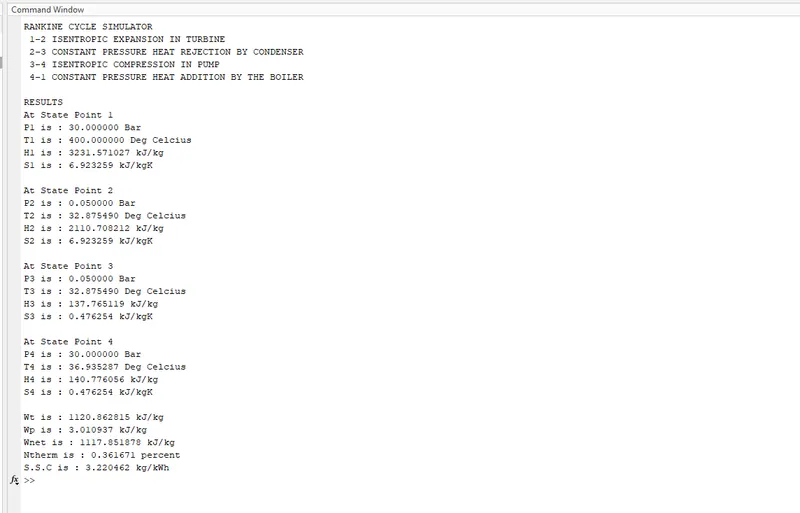
b. TS Diagram of the cycle: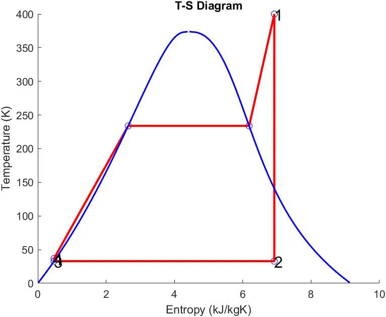
c. HS Diagram: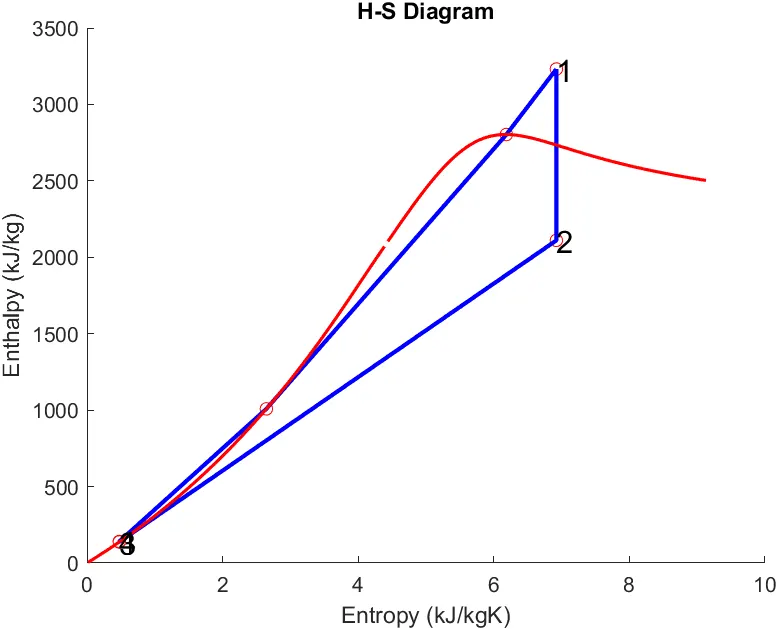
- Errors: The errors that I faced were majorly the typos and the parantheses while using specific commands. So, when MATLAB pointed out an error, I checked for the line number and then checked for any typos and corrected them right away.
- Conclusions: In conclusion, I would like to state that this Project helped me understand the basics of a Rankine Cycle and how to calculate the various Thermodynamic Properties at the four different state points as well.