Challenge

Project 2 - Rankine cycle Simulator

MMalik Zaid29 Sept 2020

Aim: to create a Rankin cycle simulator that calculate a state point variables at different points and plot the corresponding T-S and H-S plots for the given set of inputs.

Objective:

to simulate a rankine cycle using Matlab's.
extracting steam and water property from XSteam data.
calculate all the state points of the cycle based on user input.
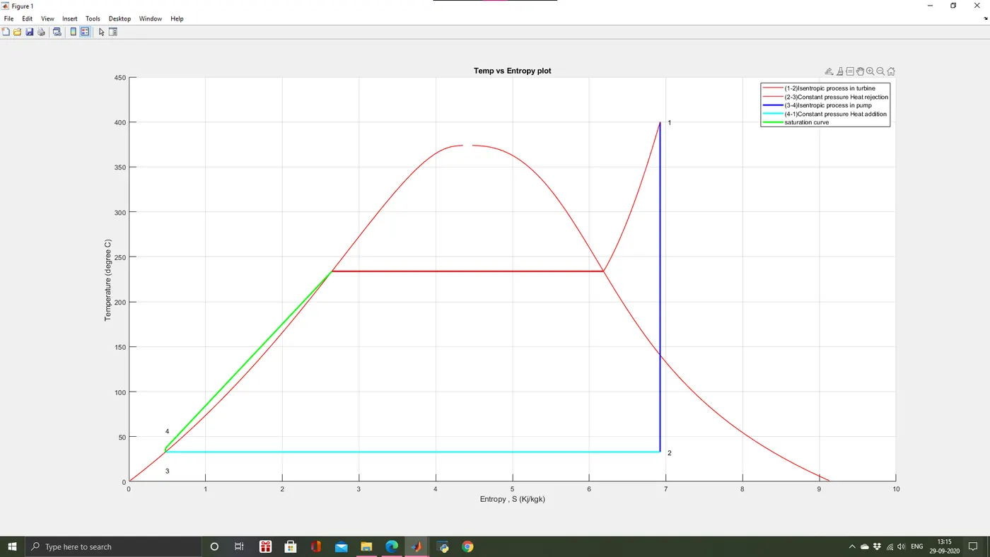
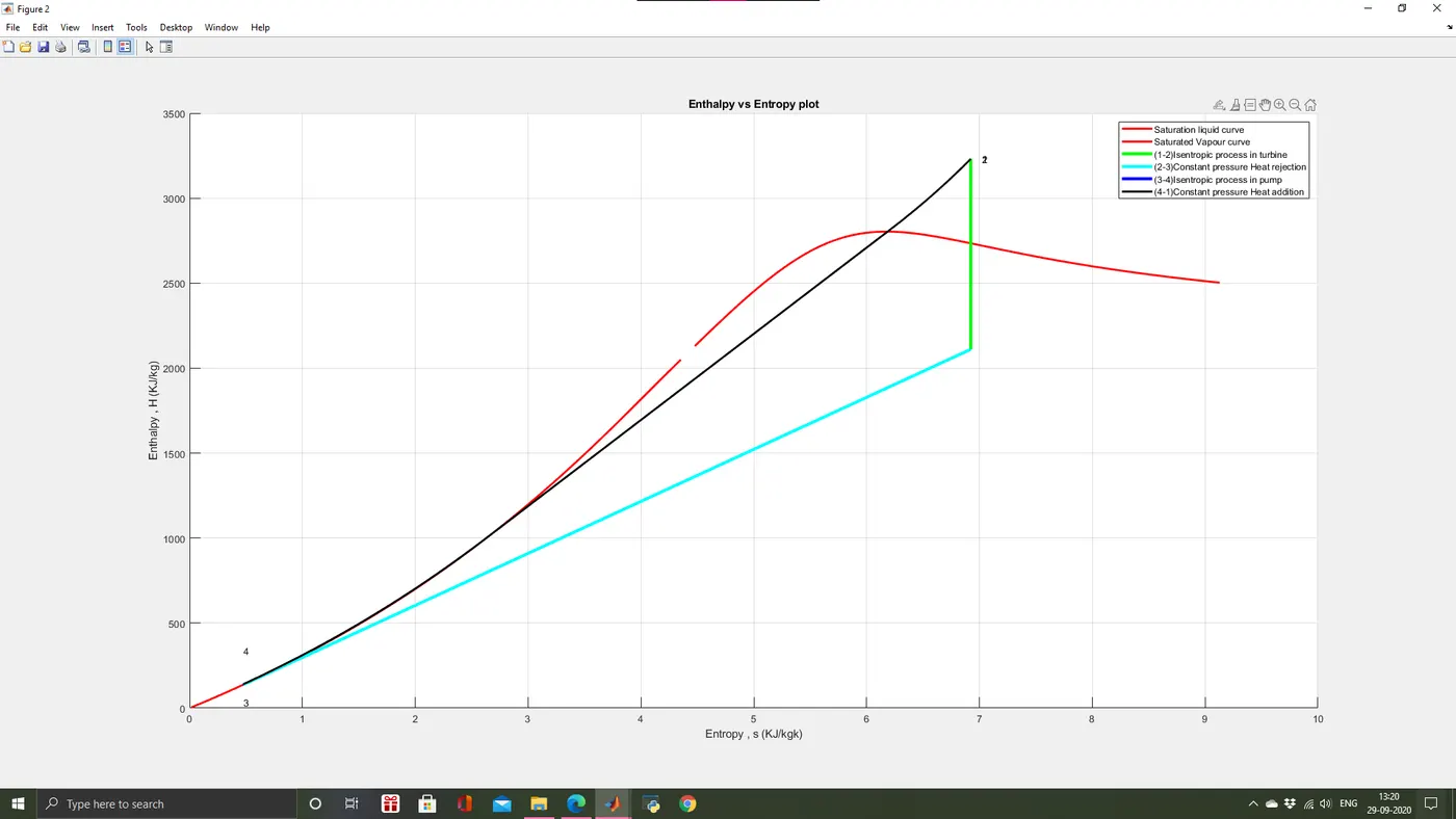
Noting that T vs s and H vs s plot for the given input.

Rankine cycle: The Rankine cycle is a model used to predict the performance of steam turbine systems. It was also used to study the performance of reciprocating steam engines. The Rankine cycle is an idealized thermodynamic cycle of a heat engine that converts heat into mechanical work while undergoing phase change. It is an idealized cycle in which friction losses in each of the four components are neglected. The heat is supplied externally to a closed loop, which usually uses water as the working fluid. It is named after William John Macquorn Rankine, a Scottish polymath and Glasgow University professor.

The Rankine cycle closely describes the process by which steam-operated heat engines commonly found in thermal power generation plants generate power.

Power depends on the temperature difference between a heat source and a cold source. The higher the difference, the more mechanical power can be efficiently extracted out of heat energy, as per Carnot's theorem.

The heat sources used in these power plants are usually nuclear fission or the combustion of fossil fuels such as coal, natural gas, and oil, or concentrated solar power. The higher the temperature, the better.

The efficiency of the Rankine cycle is limited by the high heat of vaporization of the working fluid. Also, unless the pressure and temperature reach super critical levels in the steam boiler, the temperature range the cycle can operate over is quite small: steam turbine entry temperatures are typically around 565 °C and steam condenser temperatures are around 30 °C.^{[citation needed]} This gives a theoretical maximum Carnot efficiency for the steam turbine alone of about 63.8% compared with an actual overall thermal efficiency of up to 42% for a modern coal-fired power station. This low steam turbine entry temperature (compared to a gas turbine) is why the Rankine (steam) cycle is often used as a bottoming cycle to recover otherwise rejected heat in combined-cycle gas turbine power stations.

The cold source (the colder the better) used in these power plants are usually cooling towers and a large water body (river or sea). The efficiency of the Rankine cycle is limited on the cold side by the lower practical temperature of the working fluid.

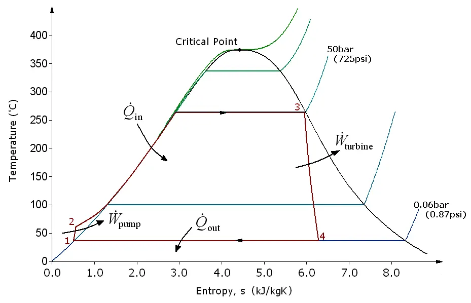
The working fluid in a Rankine cycle follows a closed loop and is reused constantly. The water vapor with condensed droplets often seen billowing from power stations is created by the cooling systems (not directly from the closed-loop Rankine power cycle). This 'exhaust' heat is represented by the "Q_out" flowing out of the lower side of the cycle shown in the T–s diagram below. Cooling towers operate as large heat exchangers by absorbing the latent heat of vaporization of the working fluid and simultaneously evaporating cooling water to the atmosphere.

While many substances could be used as the working fluid in the Rankine cycle, water is usually the fluid of choice due to its favorable properties, such as its non-toxic and unreactive chemistry, abundance, and low cost, as well as its thermodynamic properties. By condensing the working steam vapor to a liquid the pressure at the turbine outlet is lowered and the energy required by the feed pump consumes only 1% to 3% of the turbine output power and these factors contribute to a higher efficiency for the cycle. The benefit of this is offset by the low temperatures of steam admitted to the turbine(s). Gas turbines, for instance, have turbine entry temperatures approaching 1500 °C. However, the thermal efficiency of actual large steam power stations and large modern gas turbine stations are similar.

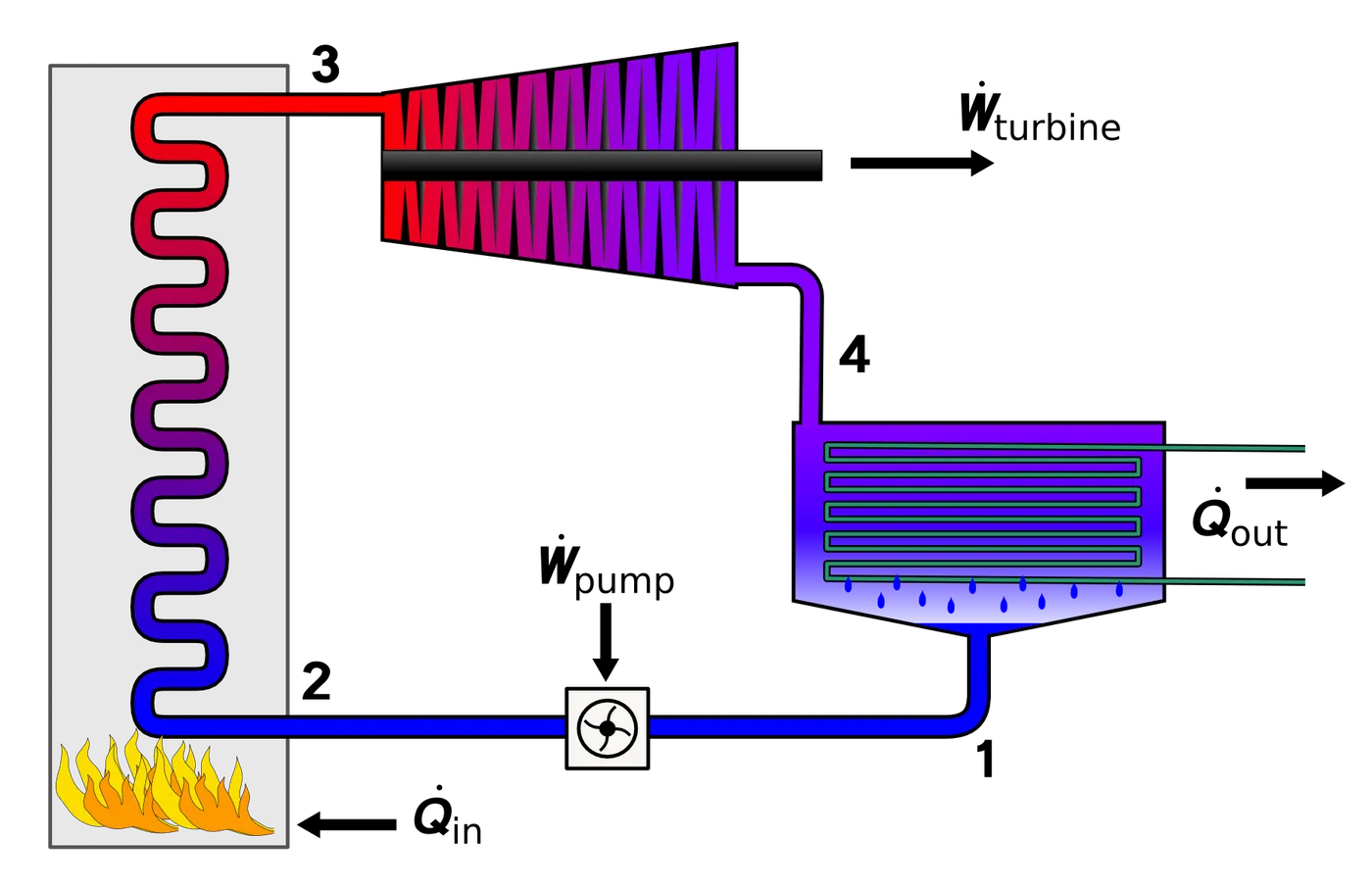
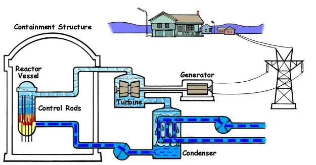
The four processes in the Rankine cycle:

There are four processes in the Rankine cycle. The states are identified by numbers (in brown) in the T–s diagram.

Process 1–2: The working fluid is pumped from low to high pressure. As the fluid is a liquid at this stage, the pump requires little input energy.

In other words Process 1-2 is [Isentropic compression]

Process 2–3: The high-pressure liquid enters a boiler, where it is heated at constant pressure by an external heat source to become a dry saturated vapour. The input energy required can be easily calculated graphically, using an enthalpy–entropy chart (h–s chart, or Mollier diagram), or numerically, using steam tables.

In other words Process 2-3 is [Constant pressure heat addition in boiler]

Process 3–4: The dry saturated vapour expands through a turbine, generating power. This decreases the temperature and pressure of the vapour, and some condensation may occur. The output in this process can be easily calculated using the chart or tables noted above.

In other words Process 3-4 is [Isentropic expansion]

Process 4–1: The wet vapour then enters a condenser, where it is condensed at a constant pressure to become a saturated liquid.

In other words Process 4-1 is [Constant pressure heat rejection in condenser]

main program:

XSteam Data is used to extract steam and water properties of enthalpy entropy and specific pressure and temperatures for sat liquid sat vapour conditions etc
The program requires the input of pressure (in bars) at state point 1 (turbine inlet) temperature at same point (degrees Celsius) and temperature at condenser inlet point 2
With the help of these inlets and form XSteam Data the program calculates all the state points of Rankine cycle
the XSteam data works as
h1=XSteam('h_pT,p1,T1') (returns the enthalpy of water at a given pressure and temperature in bars and degree respectively)
as we extract the data we use thermodynamics relation to further find statements and extract the data from XSteam
sf and sg , hf and hg where f and g stands for saturated liquid and saturated vapour respectively
The network work done by turbine work done by run the pump heat in And heat out or calculated using standard thermodynamics Relationship
efficiency and specific steam consumption (s.s.c) Of Rankine cycle is calculated
T,s and h are extracted at vapour and liquid line for plotting purpose after 4th point for the variation you observe in the plot
saturation curve is plotted in red for saturated liquid and saturated gas.
plot T vs s and h vs s is created from all the points obtained from the program
the plot change as the user input changes for the above mentioned inputs
results are displayed in the command window

Explanation of the code:

As mentioned above regarding the process takes place in rankine cycle all the process first displayed using 'disp' command
The user is then asked to input the value of inlet pressure inlet temperature outlet pressure of turbine and this can be achieved using 'input' command
The state point variable or now calculated using the XSteam function file By passing it a correct set of input arguments
The state properties like temperature enthalpy specific entropy of liquid vapour superheated steam or calculated at the respective state points
finally the thermodynamics process are plotted using plot command
at the end of the program the result this or displayed to the user which displays all the state variables a different state points and this was achieved using fprintf commad

%% Rankine cycle simulator
% object of this programis to simulate  the rankine cycle 
% plotting t-s and h-s diagram using data from XSteam data
%water and steam properties according to IAPWS IF-97
close all
clear all
clc

%%
disp('RANKINE CYCLE');
disp('1-2 is Isentropic Expansion in the turbine');
disp('2-3 is Constant Pressure Heat is Rejection by the condensor');
disp('3-4 is Isentropic Compression in the pump');
disp('4-1 is Constant Pressure Heat Addition by the boiler');


%%
%OBTAINING THE INPUT VALUE 
p1 = input('nValue of Pressure at the Turbine inlet,p1(in bar) = ');
T1 = input('nValue of Temperature at Turbine inlet,T1(in degree.c) = ');
p2 = input('nValue of Temperature at condensor inlet, p2(in bar) = ');

%%
%Extracting data_defining variables
%state 1

h1 = XSteam('h_pT',p1,T1);  %EXTRACTING ENTHALPY AT STATE 1
s1 = XSteam('S_pT',p1,T1);   %SIMILARLY


% STATE 2

s2 = s1;                        %iSENTROPIC EXPENSION   
sf2 = XSteam('sL_p',p2);         %Saturated liquid entropy
sg2 = XSteam('sV_p',p2);          %Saturated vapour entropy
x2 = (s2-sf2)/(sg2-sf2);
hf2 = XSteam('hL_p',p2);
hg2 = XSteam('hV_p',p2);
h2 = hf2+ (x2*(hg2-hf2));

 % STATE 3
 p3 = p2;                       %constant pressure heat rejection in cindenser 
 s3 = XSteam('sL_p',p3);
 h3 = XSteam('hL_p',p3);
 
 % STATE 4
 s4 = s3;
 p4 = p1;
 
 %%
 %work done by turbine
 Wt = h1-h2;
 
% work done to run pump
v3 = XSteam('vL_p',p3);
Wp = v3*(p4 - p3)*100;
h4 = h3 + Wp;

%net work
Wnet = Wt -Wp;

%Heat into  the system
Qin = h1 - h4;

%Heat out of the system
Qout = h2 - h3;

%Thermal efficiency
eff = (Wnet/Qin)*100;

%Specific steam consumption
%SSC = mass flow rate/power
SSC = (3600/Wnet);

%%
%Calculating temperature at the state points
T3 = XSteam('Tsat_p',p3);
T2 = T3;
Cp4 = XSteam('Cp_ps',p4,s4);
Cv4 = XSteam('Cv_ps',p4,s4);
k = Cp4/Cv4;
T4 = T3/((p3/p4)^((k-1)/k));

%Calculating temperature,entropy and enthlpy at the vapour and liquid
%line for ploting
T6 = XSteam('Tsat_p',p1);
s5 = XSteam('sL_p',p1);
s6 = XSteam('sV_p',p1);
h5 = XSteam('hL_p',p1);
h6 = XSteam('hV_p',p1);
T5 = T6;

%%
%Plotting the saturation curves
T = linspace(1,375,1000);
for i = 1:length(T)
    
    sf(i) = XSteam('sL_T',T(i));
    sg(i) = XSteam('sV_T',T(i));
    hf(i) = XSteam('hL_T',T(i));
    hg(i) = XSteam('hV_T',T(i));
end
%Plotting T-s diagram
figure(1)
grid on
hold on
plot(sf,T,'linewidth',1,'color','r')
plot(sg,T,'linewidth',1,'color','r')
plot([s1 s2],[T1 T2],'linewidth',2,'color','b')
plot([s2 s3],[T2 T3],'linewidth',2,'color','c')
plot([s3 s4],[T3 T4],'linewidth',2,'color','g')
plot([s4 s5],[T4 T5],'linewidth',2,'color','g')
plot([s5 s6],[T5 T6],'linewidth',2,'color','r')
sc1 = linspace(s6, s1, 1000);
for l = 1:length(sc1)
    Tc1(l) = XSteam('T_ps',p1,sc1(l));
end

plot(sc1, Tc1,'linewidth',1,'color','r')
text(s1+0.1,T1, '1')
text(s2+0.1,T2, '2')
text(s3,T3-20, '3')
text(s4,T4+20 ,'4')
title('Temp vs Entropy plot')
xlabel('Entropy , S (Kj/kgk)')
ylabel('Temperature (degree C) ')
legend('(1-2)Isentropic process in turbine','(2-3)Constant pressure Heat rejection','(3-4)Isentropic process in pump','(4-1)Constant pressure Heat addition','saturation curve')

%%
%Plotting h-s diagram
figure(2)
grid on
hold on
plot(sf, hf, 'r','linewidth',2,'color','r')
plot(sg, hg, 'r','linewidth',2,'color','r')
plot([s1 s2],[h1 h2],'k','linewidth',3,'color','g')
plot([s2 s3],[h2 h3],'k','linewidth',3,'color','c')
plot([s3 s4],[h3 h4],'k','linewidth',3,'color','b')
hc = linspace(h4, h5, 100)
 
for k = 1:length (hc)
    sch(k) = XSteam('s_ph',p1,hc(k))

end
plot(sch,hc,'k','linewidth',2)
plot([s5 s6],[h5 h6],'k','linewidth',2)

for m = 1:length(sc1)
    hc1(m) = XSteam('h_ps',p1,sc1(m));
end

plot(sc1,hc1,'k', 'linewidth',2)
text(s1+0.1,h1,'1')
text(s2+0.1,h1,'2')
text(s3,h3-100,'3')
text(s4,h4+200,'4')
title('Enthalpy vs Entropy plot')
xlabel('Entropy , s (KJ/kgk)')
ylabel('Enthalpy , H (KJ/kg)')
legend('Saturation curve','location','northwest')

%%
%Displaying Result
disp('RESULTS');
fprintf('At State Point 1:n');
fprintf('p1: %8.3f barn',p1);
fprintf('T1: %8.3f Cn',T1);
fprintf('h1: %8.3f KJ/kgk',h1);
fprintf('s1: %8.3f KJ/kgknn',s1);
fprintf('At State Point 2:n');
fprintf('p2: %8.3f barn',p2);
fprintf('T2: %8.3f Cn',T2);
fprintf('h2: %8.3f KJ/kgk',h2);
fprintf('s2: %8.3f KJ/kgknn',s2);
fprintf('x2: %8.3fnn',x2);
fprintf('At State Point 3:n');
fprintf('p3: %8.3f barn',p3);
fprintf('T3: %8.3f Cn',T3);
fprintf('h3: %8.3f KJ/kgk',h3);
fprintf('s3: %8.3f KJ/kgknn',s3);
fprintf('At State Point 4:n');
fprintf('p4: %8.3f barn',p4);
fprintf('T4: %8.3f Cn',T4);
fprintf('h4: %8.3f KJ/kgk',h4);
fprintf('s4: %8.3f KJ/kgknn',s4);
fprintf('Turbine Work: %8.3f kJ/kgn',Wt);
fprintf('Pump Work: %8.3f kJ/kgn',Wp);
fprintf('Wnet: %8.3f kJ/kgn',Wnet);
fprintf('Efficiency: %8.3f percent n',eff);
fprintf('S.S.C: %8.3F kJ/kWh',SSC);

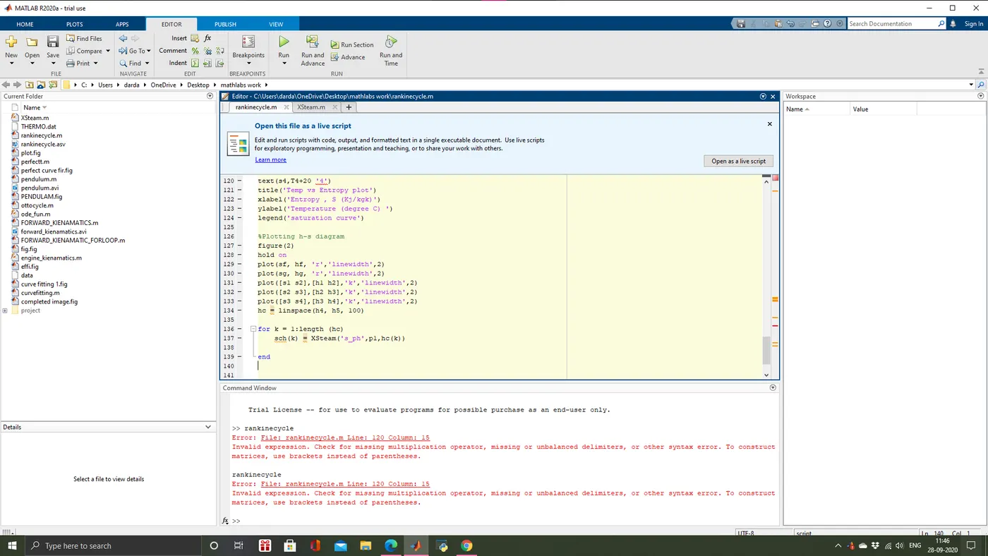
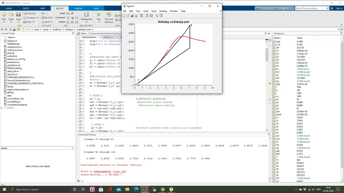
Errors during program i got: