Project 2 - Rankine cycle Simulator
Aim:
To Create a Rankine Cycle Simulator using OCTAVE/MATLAB.
Software Used:
MATLAB R2020
Theory:
Schematic of Rankine Cycle:
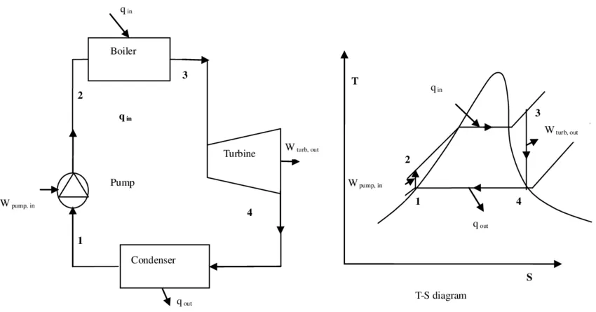
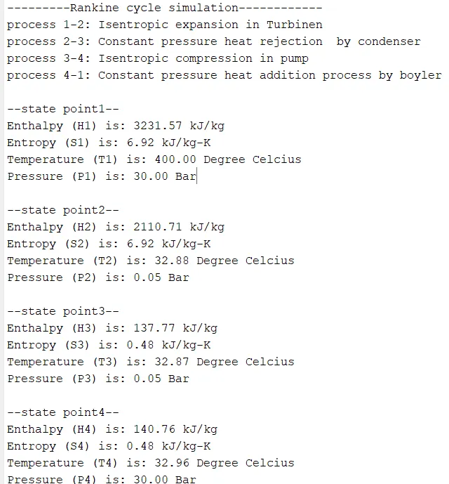
process 1-2: Isentropic expansion in Turbinen
process 2-3: Constant pressure heat rejection by condenser
process 3-4: Isentropic compression in pump
process 4-1: Constant pressure heat addition process by boyler
Governing equations:
Heat Supplied:
`Qadd`= `H1-H4`
Heat Rejected:
`Qout`= `H2-H3`
Turbine Work:
`Wt`= `H1-H2`
Pump Work:
`Wp`= `H4-H3`
Net Work done:
`W`= `Wt-Wp`
Efficiency of Rancine Cycle:
`eta``W/(Qadd)`
Back work Ratio;
`B W R= (Wp)/(Wt)`
Specific Steam Consumption:
`SSC`= `3600/(Wt)`
Where,
`T= Temperature` `K`
`P=Pressure` `Bar`
`H`= `Enthalpy` `(kJ)/(kg)`
`S= Entropy` `(kJ)/(kg-K)`
MATLAB CODE:
%Rankine cycle
clear all
close all
clc
fprintf('---------Rankine cycle simulation------------n');
%printing all the four processes in Rankin cycle.
fprintf('process 1-2: Isentropic expansion in Turbinenn');
fprintf('process 2-3: Constant pressure heat rejection  by condensern');
fprintf('process 3-4: Isentropic compression in pumpn');
fprintf('process 4-1: Constant pressure heat addition process by boylernn');

%Getting the thermodynamic properties
%pressure (P1) at turbine inlet
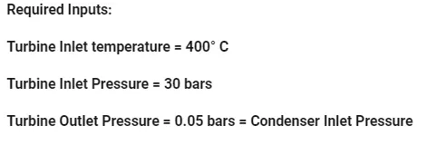
P1=30;
%Pressure (P2) at condenser inlet
P2=0.05;
%Temperature (T1) at turbine inlet
T1=400;

%Calculating the thermodynamic properties in all four state points
%At state point 1
%Enthalpy(H1)
H1=XSteam('h_pt',P1,T1);
%Entropy(S1)
S1=XSteam('s_pt', P1,T1);

%At state point 2
%Entropy(S2)
S2=S1; %Isentropic process
%Calculating X2
Sf2= XSteam('sL_p',P2);
Sg2= XSteam('sV_p',P2);
hf2= XSteam('hL_p',P2);
hgf2= XSteam('hV_p',P2);
x2= ((S2-Sf2)/(Sg2-Sf2));

%Enthalpy(H2)
H2= (hf2+(x2*(hgf2-hf2)));
%Temperature(T2)
T2= XSteam('T_Ps', P2,S2);

%At state point 3
%Pressure (P3)
P3=P2;
%Entropy (S3)
S3=XSteam('sL_p', P3);
%Temperature(T2)
T3= XSteam('T_Ps', P3,S3);
%Calculating X3
Sf3= XSteam('sL_p',P3);
Sg3= XSteam('sV_p',P3);
hf3= XSteam('hL_p',P3);
hgf3= XSteam('hV_p',P3);
x3= ((S3-Sf3)/(Sg3-Sf3));

%Enthalpy (H3)
H3=(hf3+(x3*(hgf3-hf3)));

%At state point 4
%Entropy (S4)
S4=S3; %Isentropic process
%Pressure(P4)
P4=P1; %Constant pressure heat addition process
%Enthalpy(H4)
H4= XSteam('h_ps',P4,S4);
%Temperature(T4)
T4=XSteam('T_hs',H4,S4);

%State point 5
%Temperature(T5)
T5=XSteam('Tsat_p',P4);
%Entropy(S5)
S5=XSteam('sL_p',P4);

%At state point 6
%Temperature(T6)
T6= T5;
%Entropy(S6)
S6= XSteam('sV_T',T6);

%Rankine Cycle parameters
%Turbine work(Wt)
Wt=H1-H2;
%Pump work(Wp)
Wp=H4-H3;
%Net work done
Wnet=Wt-Wp;
%Heat suppled(Qin)
Qin=H1-H4;
%Heat rejected(Qout)
Qout=H2-H3;

%Efficiency of Rankin cycle(Eff)
Eff=(Wnet/Qin)*100;

%Back work ratio(BWR)
BWR=(Wp/Wt);

%Specific steam consumption(SSC)
SSC=(3600/Wt);

%Printing the evaluated parameters
%State point1
fprintf('--state point1--n');
fprintf('Enthalpy (H1) is: %0.2f kJ/kgn',H1);
fprintf('Entropy (S1) is: %0.2f kJ/kg-Kn',S1);
fprintf('Temperature (T1) is: %0.2f Degree Celciusn',T1);
fprintf('Pressure (P1) is: %0.2f Barnn',P1);

%State point2
fprintf('--state point2--n');
fprintf('Enthalpy (H2) is: %0.2f kJ/kgn',H2);
fprintf('Entropy (S2) is: %0.2f kJ/kg-Kn',S2);
fprintf('Temperature (T2) is: %0.2f Degree Celciusn',T2);
fprintf('Pressure (P2) is: %0.2f Barnn',P2);

%State point3
fprintf('--state point3--n');
fprintf('Enthalpy (H3) is: %0.2f kJ/kgn',H3);
fprintf('Entropy (S3) is: %0.2f kJ/kg-Kn',S3);
fprintf('Temperature (T3) is: %0.2f Degree Celciusn',T3);
fprintf('Pressure (P3) is: %0.2f Barnn',P3);

%State point4
fprintf('--state point4--n');
fprintf('Enthalpy (H4) is: %0.2f kJ/kgn',H4);
fprintf('Entropy (S4) is: %0.2f kJ/kg-Kn',S4);
fprintf('Temperature (T4) is: %0.2f Degree Celciusn',T4);
fprintf('Pressure (P4) is: %0.2f Barnn',P4);

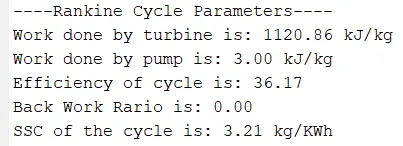
fprintf('----Rankin Cycle Parameters----n')
%Turbine work(Wt)
fprintf('Work done by turbine is: %0.2f kJ/kgn',Wt);
%Pump work(Wp)
fprintf('Work done by pump is: %0.2f kJ/kgn',Wp);
%Efficiency
fprintf('Efficiency of cycle is: %0.2fn',Eff);
%Back Work Ratio
fprintf('Back Work Rario is: %0.2fn',BWR);
%SSC
fprintf('SSC of the cycle is: %0.2f kg/KWhnn',SSC);

%Plotting
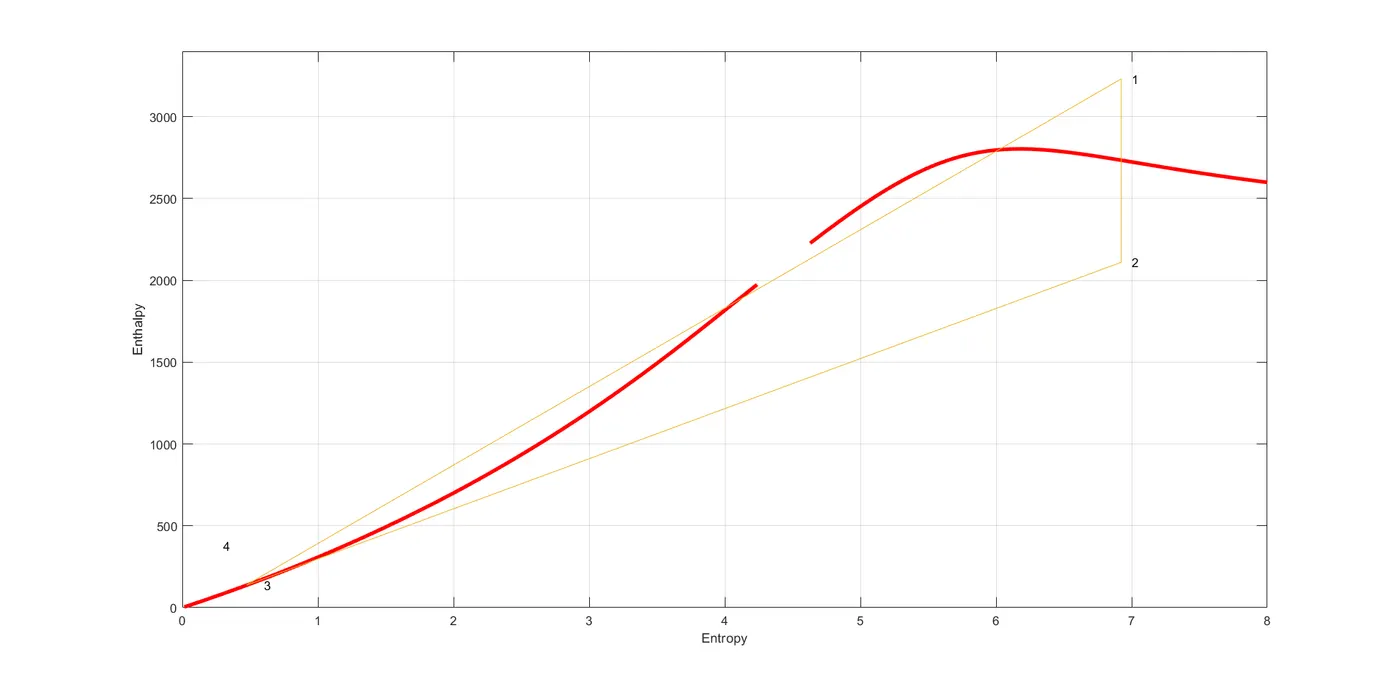
%H-S Diagram
%points for saturation curve
s_c= (1:1000);
for i= 1:1000
    s_l(i)= XSteam('sL_T',i);
    h_l(i)= XSteam('hL_T',i);
    s_v(i)= XSteam('sV_T',i);
    h_v(i)= XSteam('hV_T',i);
end

%Saturation curve
figure(1)
plot(s_l,h_l,'linewidth',3,'color','r');
hold on
plot(s_v, h_v,'linewidth',3,'color','r');

%State point1
plot([S1 S2 S3 S4 S1],[H1 H2 H3 H4 H1]);
text(7,H1,'1');
text(7,H2,'2');
text(0.6,H3,'3');
text(0.3,380,'4');
ylim([0 3400])
xlim([0 8])
xlabel('Entropy')
ylabel('Enthalpy')
grid on
hold off

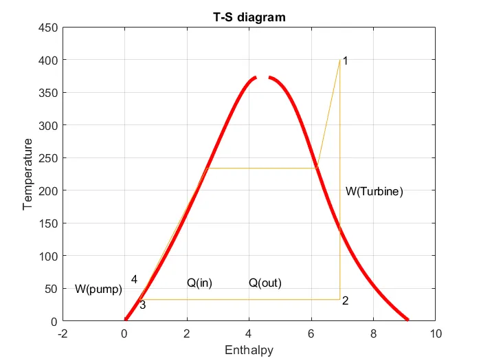
%T-S diagram
%Saturation curve
figure(2)
plot(s_l,s_c,'-','linewidth',3,'color','r')
hold on
plot(s_v,s_c,'-','linewidth',3,'color','r')

%State points
plot([S1 S2 S3 S4 S5 S6 S1],[T1 T2 T3 T4 T5 T6 T1])
text(7,T1,'1');
text(7,T2,'2');
text(S3,26,'3');
text(0.2,65,'4');
text(7.1,200,'W(Turbine)');
text(4,60,'Q(out)');
text(2,60,'Q(in)');
text(-1.6,50,'W(pump)');
ylim([0 450])
xlim([-2,10])
xlabel('Enthalpy')
ylabel('Temperature')
title('T-S diagram')
grid on
hold off
Procedure:
- Initially required input values are defined.
- Then, calculated the thermodynamic properties (`T`, `P`, `H`, `S`,`Wt`,`Wp`, `W` `eta`, `BWR`, `SSC`) in all the six state points by referring the XSteam Library Data.
- After calcutaion, printed the results to display in the command window.
- Next, plotted the T-S diagram & H-S diagram, by providing all the required labelings and titles.
- After programming, the code was run, by that the code get complied and printed the results and plots at the end terminated.
Output:
- Plots
Results:
Data file:
Xsteam Library