Project 2 - Rankine cycle Simulator

AIM:

To simulate the Rankine Cycle using MATLAB.

OBJECTIVE:

• Calculate the state points of the Rankine cycle based on user inputs.
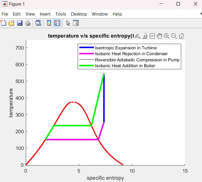
• Plot the corresponding T-S and H-S plots for the given set of inputs.
• Calculate cycle efficiency and back work ratio.

THEORY:

• The Rankine cycle or Rankine Vapor Cycle is the process widely used by power plants such as coal-fired power plants or nuclear reactors.
• In this mechanism, a fuel is used to produce heat within a boiler, converting water into steam which then expands through a turbine producing useful work.
• This process was developed in 1859 by Scottish engineer William J.M. Rankine.
• This is a thermodynamic cycle which converts heat into mechanical energy—which usually gets transformed into electricity by electrical generation.

RANKINE CYCLE:

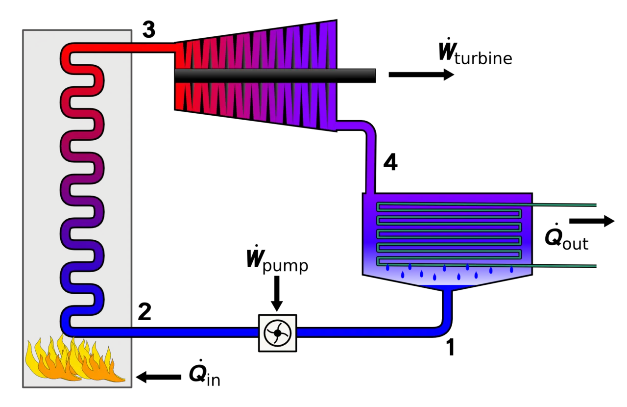
1. P-V PLOT

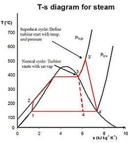
2. H-S PLOT

There are four processes in the Rankine cycle. The states are identified by numbers (in brown) in the T–s diagram.

PROCESS1-2: The dry saturated vapour expands through a turbine, generating power. This decreases the temperature and pressure of the vapour, and some condensation may occur.

In other words Process 1-2 is, Isentropic expansion.

PROCESS 2-3: The wet vapour then enters a condenser, where it is condensed at a constant pressure to become a saturated liquid.

In other words Process 2-3 is, Constant pressure heat rejection in condenser.

PROCESS 3-4: The working fluid is pumped from low to high pressure. As the fluid is a liquid at this stage, the pump requires little input energy.

In other words Process 3-4 is, Isentropic compression.

PROCESS 4-1: The high-pressure liquid enters a boiler, where it is heated at constant pressure by an external heat source to become a dry saturated vapour. The input energy required can be easily calculated graphically, using an enthalpy–entropy chart (h–s chart, or Mollier diagram), or numerically, using steam tables.

In other words Process 4-1 is, Constant pressure heat addition in boiler.

• In an ideal Rankine cycle the pump and turbine would be isentropic, i.e., the pump and turbine would generate no entropy and hence maximize the net work output.
• Processes 1–2 and 3–4 are represented by vertical lines on the T–S diagram.
• The efficiency of the Rankine cycle is limited by the high heat of vaporization by the fluid.
• The fluid must be cycled through and reused constantly, therefore, water is the most practical fluid for this cycle.
• This is not why many power plants are located near a body of water—that's for the waste heat.
• As the water condenses in the condenser, waste heat is given off in the form of water vapour—which can be seen billowing from a plant's cooling towers.
• This waste heat is necessary in any thermodynamic cycle.
• Due to this condensation step, the pressure at the turbine outlet is lowered.
• This means the pump requires less work to compress the water—resulting in higher overall efficiencies.

EQUATIONS :

1. Work _turbine,out = h₁ – h₂ : Work done (Output work) by turbine in process 1-2.
2. Q _in = h₁ – h₄ : Heat given to the system in boiler, process 4-1.
3. Work _pump,in = h₄ – h₃ : Work done by pump (Input work) in process 3-4.
4. Q _out = h₂ – h₃ : Heat released by the system in condenser, process 2-3.
5. Work _Shaft = Work _net = Work _turbine,out - Work _pump,in : Net work done which is the work done by shaft.
6. The thermal efficiency of the Rankine cycle is determined from:

`η t h = Work s h a f t Q in ⋅ 100 = ( 1 − Q o u t Q in ) ⋅ 100`

PROGRAM:

clear all
close all
clc
% Rankine cycle-PROJECT 2
f = fopen("XSteam.m","r")

% Printing the heading 
fprintf('RANKINE CYCLE STIMULATOR \n')
disp('process 1-2:isentropic expansion in turbine')
disp('2-3:constant pressure heat rejection by the condensor')
disp('3-4:isentropic compression in pump')
disp('4-1:constant pressure heat addition in boiler')

% Giving the initial inputs by the user
% P1 = Inlet pressure of turbine(bar)
% P2 = outlet pressure of turbine(bar)
% T1 = Inlet temp of turbine(celsius)

fprintf('\n')
p1 = input('enter pressure at turbine inlet: ');
p2 = input('enter pressure at turbine outlet: ');
t1 = input('enter temperature at turbine inlet: ');

% calculating various parameters for rankine cycle
% h = Enthalpy
% s = Entropy
% t = Temperature
% p = pressure
% v = volume

% calculating state variable at point 1
h1 = XSteam('h_pT',p1,t1);
s1 = XSteam('s_pT',p1,t1);
hf1 = XSteam('hL_p',p1); 
hg1 = XSteam('hV_p',p1);
ts1 = XSteam('Tsat_p',p1);
sf1 = XSteam('sL_p',p1);
sg1 = XSteam('sV_p',p1); 

% calculating state variable at point 2
s2 = s1; % process 1-2 is isentropic expansion in turbine
sf2 = XSteam('sL_p',p2); 
sg2 = XSteam('sV_p',p2); 
x = (s2-sf2)/(sg2-sf2); 
hf2 = XSteam('hL_p',p2);
hg2 = XSteam('hV_p',p2);
h2 = hf2+x*(hg2-hf2); 
t2 = XSteam('T_ph',p2,h2);
ts2 = XSteam('Tsat_p',p2);

% calculating state variables at point 3
h3 = hf2; 
s3 = sf2; 
t3 = t2 ; 
p3 = p2; 

% calculating state variables at point 4
p4 = p3 ; % Process 4-1 pressure heat addition 
s4 = s3; % process 3-4 isentropic compression
h4 = XSteam('h_ps',p4,s4); 
t4 = XSteam('T_ps',p4,s4); 

% Temp space for plotting saturation curves
t = linspace(0,380,500);

% plot T-S diagram
figure(1)
hold on
% plotting the saturation curve
for i = 1:length(t)
   plot(XSteam('sL_T',t(i)),t(i),'.','color','r')   
   plot(XSteam('sV_T',t(i)),t(i),'.','color','r') 
end

% Plotting the rankine cycle
a1 = plot([s1 s2],[t1 t2],'LineWidth',3,'Color','b');
if x>1
    t3 = ts2;
    a2 = plot([s2 sg2 s3],[t2 ts2 t3],'LineWidth',3,'Color','m');
    t2 =ts2;
else
    a2 = plot([s2 s3],[t2 t3],'LineWidth',3,'Color','m');
end
a3 = plot([s3 s4],[t3 t4],'Color','k');
a4 = plot([s4 sf1 sg1 s1],[t4 ts1 ts1 t1],'LineWidth',3,'Color','g');

axis([0 15 -5 (t1+200)])
xlabel('specific entropy')
ylabel('temperature')
legend([a1 a2 a3 a4],{'Isentropic Expansion in Turbine','Isobaric Heat Rejection in Condenser','Reversible Adiabatic Compression in Pump ','Isobaric Heat Addition in Boiler'},'location','northeast');
title('temperature v/s specific entropy(t-s diagram)')
hold off

% plotting for h-s diagram
figure(2)
hold on

% plotting the saturation curve
for i = 1:length(t)
    plot(XSteam('sL_T',t(i)),XSteam('hL_T',t(i)),'.','Color','g')
    plot(XSteam('sV_T',t(i)),XSteam('hv_T',t(i)),'.','Color','r')
end

% plotting the rankine cycle
A1 = plot([s1 s2],[h1 h2],'LineWidth',2,'Color','b');
A2 = plot([s2 s3],[h2 h3],'LineWidth',2,'Color','g');
A3 = plot([s3 s4],[h3 h4],'LineWidth',2,'Color','k');
A4 = plot([s4 s1],[h4 h1],'LineWidth',2,'Color','m');
xlabel('specific entropy')
ylabel('specific enthalpy')
title('Specific Enthalpy v/s Specific Entropy (H-S Diagram)')
legend([A1 A2 A3 A4],{'Isentropic Expansion in Turbine','Isobaric Heat Rejection in Condenser','Isentropic Compression in Pump','Isobaric Heat Addition in Boiler'},'location','southeast')
hold off

% calculation
% turbine work
Wt = h1-h2;

% pump work
Wp = h4-h3;
% heat addition
Qin = h1-h4;

% heat rejection
Qout = h2-h3;

% net work
Wnet = Wt-Wp;

% efficiency
Ntherm = (Wnet/Qin)*100;

% specific steam consumption
SSC = 3600/Wnet;

% Back work ratio
BWR = Wp/Wt;

% printing Results
  fprintf('\n\nResults\n')
    fprintf('Parameters at State Point 1:\n')
    fprintf('p1 is : %.2f bar\n',p1)
    fprintf('t1 is : %.2f Deg Celcius\n',t1)
    fprintf('h1 is : %.2f KJ/Kg\n',h1)
    fprintf('s1 is : %.2f KJ/Kg-K\n',s1) 
 
    fprintf('\nParameters at State Point 2:\n')
    fprintf('p2 is : %.2f bar\n',p2)
    fprintf('t2 is : %.2f Deg Celcius\n',t2)
    fprintf('h2 is : %.2f KJ/Kg\n',h2)
    fprintf('s2 is : %.2f KJ/Kg-K\n',s2) 
    fprintf('Compression ratio x is : %.2f \n',x) 
 
    fprintf('\nParameters at State Point 3:\n')
    fprintf('p3 is : %.2f bar\n',p3) 
    fprintf('t3 is : %.2f Deg Celcius\n',t3)
    fprintf('h3 is : %.2f KJ/Kg\n',h3) 
    fprintf('s3 is : %.2f KJ/Kg-K\n',s3) 
 
    fprintf('\nParameters at State Point 4:\n') 
    fprintf('p4 is : %.2f bar\n',p4) 
    fprintf('t4 is : %.2f Deg Celcius\n',t4) 
    fprintf('h4 is : %.2f KJ/Kg\n',h4) 
    fprintf('s4 is : %.2f KJ/Kg-K\n',s4) 
 
    fprintf('\nTurbine Work is : %.2f KJ/Kg\n',Wt) 
    fprintf('Pump Work is : %.2f KJ/Kg\n',Wp) 
    fprintf('Work net (Shaft Work)  is : %.2f KJ/Kg\n',Wnet) 
    fprintf('Thermal Efficiency is : %.2f percent\n',Ntherm) 
    fprintf('Specific steam consumption is : %.2f Kg/KWh\n',SSC)  
    fprintf('Back Work Ratio is : %.5f \n',BWR)

PROGRAM EXPANATION:

EXPLANATION OF THE PROGRAM:

1. We start with displaying some lines in the command window.
2. Then we ask user for the inputs. Function input() is used to provide the user input. User input includes temperature and pressure before entry to turbine and pressure after exit to turbine.
3. Now based on user inputs parameters at 4 state points are calculated. Thermodynamic parameters include enthalpy H, entropy S, temperature T, pressure P, and dryness factor X at state point 2.
4. For calculating these parameters XSteam()e. steam table MATLAB program is used. This program consists of functions for all thermodynamic properties. After calling these functions in the main script gives us thermodynamic properties based on other properties like temperature and pressure.
5. After calculating all parameters, the next objective is to calculate pump work, turbine work, net work output, back ratio, and thermal efficiency.
6. Now, we need to display all these results in the command window which is done by using command 'fprintf()'.
7. The next objective is to plot the graph for H-S and T-S. The firrst step in plotting this graph is to plot the saturation curve which is calculated using 'for' loop. Under 'for' loop, values for entropy and enthalpy are calculated over a temperature range. Plotting these calculated values, the plot of a saturation curve can is obtained. Other processes are plotted by plotting respective values of H, S, T.
8. To facilitate users to continue or end the program, we have introduced a while statement at the start of the script. Then at the end we ask the user if he wants to continue, if he chooses “Y” then the program runs again, if he chooses “N” the program stops.

RESULTS:

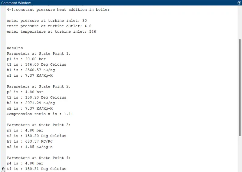
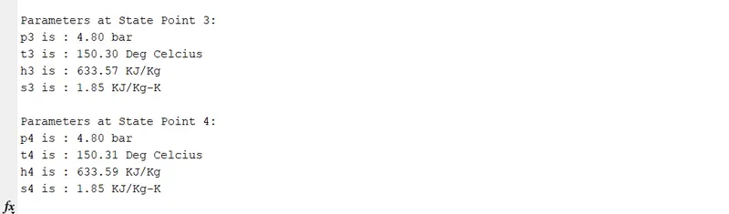
PLOTS:

T-S PLOT:

H-S PLOT:

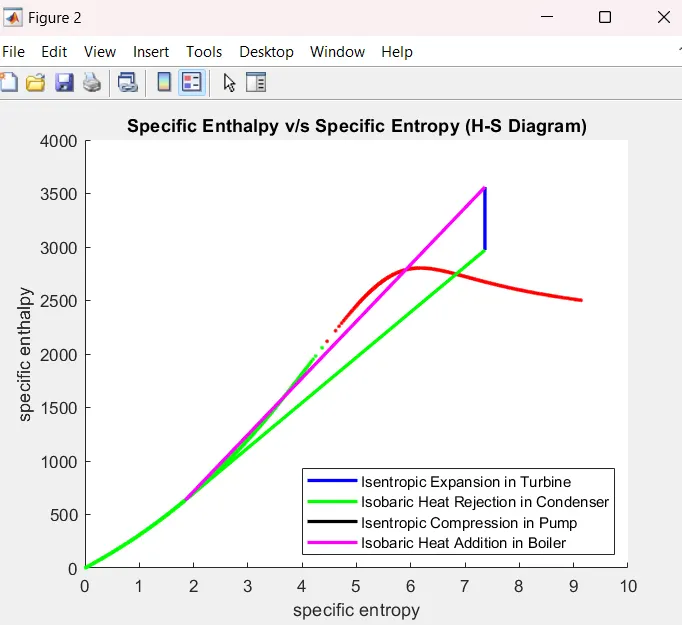
CONCLUSION:

1. For our inputs we got:

Net work output = 589.25 KJ/Kg

Back work ratio = 0.00003

2. Rankine cycle was successfully simulated by MATLAB program. For the given set of inputs we could plot the corresponding T-S and h-S plots.

REFERENCE:

http://www.ecourses.ou.edu/cgi-bin/ebook.cgi?topic=th&chap_sec=10.1&page=theory

https://en.wikipedia.org/wiki/Rankine_cycle

https://energyeducation.ca/encyclopedia/Rankine_cycle