Project - 2 - Meshing on the suspension Assembly

I. OBJECTIVES

1. To perform Geometry Clean-up on the surfaces of the given component.
2. To extract the Midsurface from the necessary component from the given model.
3. To generate shell mesh and tetra mesh on the required components with proper mesh flow.
4. To ensure that the model passes all the given mesh quality parameters.
5. To assign thickness to the midsurface coinciding with the parent geometry.
6. To create and deploy different types of connectors between various components of the given door assembly.
7. To perform the symmetry command to reflect the half-finished model to the other side.

II. CAD MODEL - REAR SUSPENSION ASSEMBLY

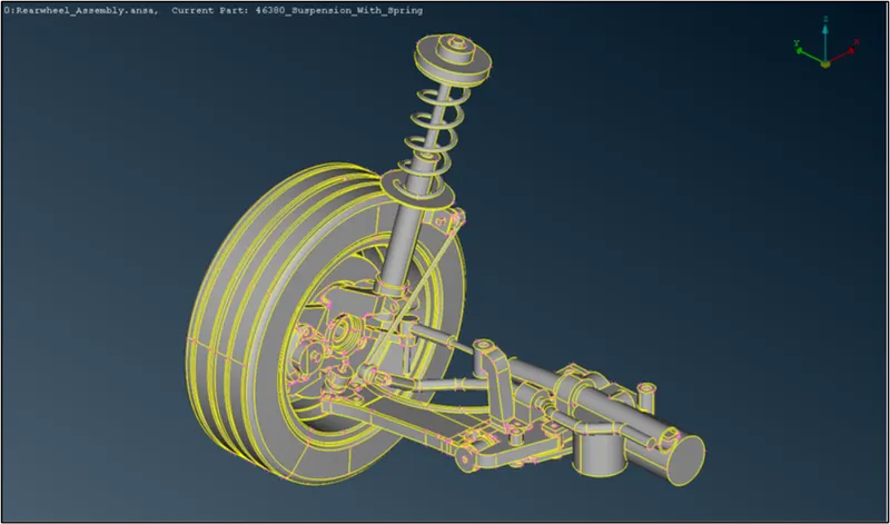Fig.1. The CAD Image of Rear Suspension Assembly

III. PARAMETERS

1. Quality Criteria for Surface Meshing of Tyre and Rim (Element type: Tria) :

   S.No	Quality Criteria	Value
   1	Target/Average length	6.5
   2	Minimum Length	5
   3	Maximum Length	10
   4	Skewness	45

2. Quality criteria for Surface Meshing of Non-Uniform thickness components other than Tyre and Rim (Element type: Tria) :

   S.No	Quality Criteria	Value
   1	Target/Average length	4
   2	Minimum Length	2
   3	Maximum Length	6
   4	Skewness	45

3. Quality Criteria for Volume meshing of all Non-Uniform thickness components (Element type: Tetra Elements):

   S.No	Quality Criteria	Value
   1	Tet-collapse	0.2

4. Quality criteria for Mid surfacing of Uniform thickness part which has a thickness less than 5 mm (Element type: Mixed elements) :

   S.No	Quality Criteria	Value
   1	Target/Average length	4
   2	Minimum Length	2
   3	Maximum Length	6
   4	Aspect	3
   5	Warpage	15
   6	Skewness	45
   7	Jacobian	0.7
   8	Minimum Quad Angle	45
   9	Maximum Quad Angle	135
   10	Minimum Tria Angle	30
   11	Maximum Tria Angle	120

IV. PROCEDURE

1. The given CAD model is imported in the ANSA window as a .ansa file as seen in Fig 1.
2. Next, there happens to be a variety of different parts in this model and shall be bifurcated in terms of their PIDs. Hence, the components are transferred to their respective PIDs once we create the required property cards. Figure 2 shows the aforementioned.

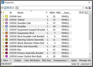
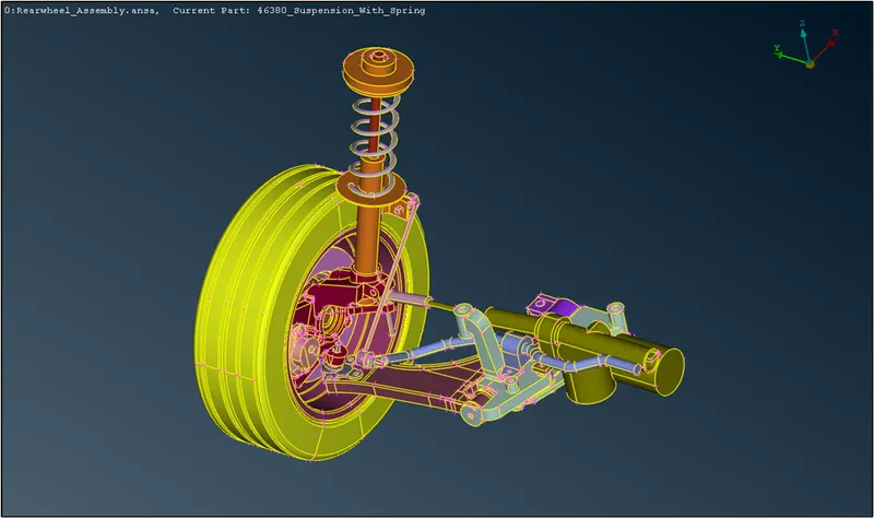
   Fig.2. Different PIDs

3. This project requires us to make use of all the important tools that we have learned till now. Hence, the procedure shall be divided as follows:

1. Extraction of Mid Surfaces and Shell mesh generation for components with thickness less than 5mm:-

1. The given model has some parts that are thinner than 5mm and shall be meshed with 2D shell mesh. The model was found to be free from any topological discrepancies. The parts are made visible and the rest are hidden.

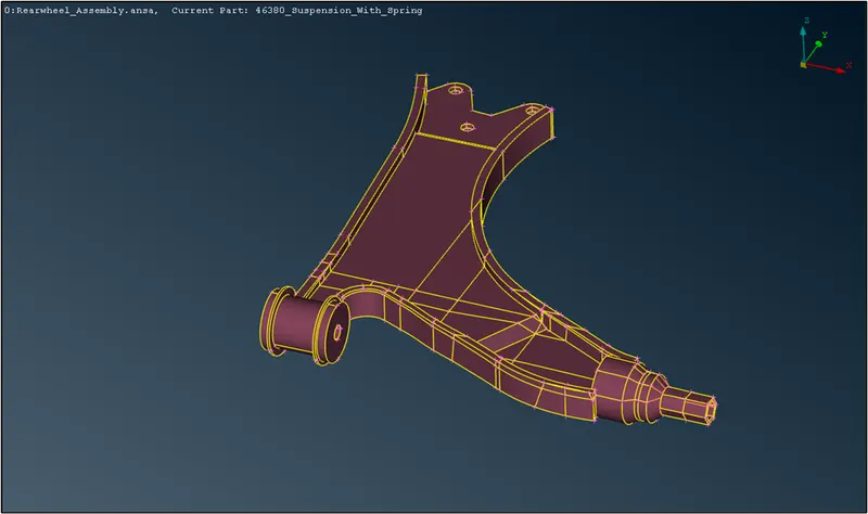
   Fig.3. Lower Control Arm for Midsurface extraction

2. The above part will be used for the midsurface extraction first. For surfaces like the top part of the model, where the middle option cannot be used, the offset option is used to get the mid surface. The thickness of the surface is first measured. Then we navigate to Topo → Faces → Offset and select the face to offset. The offset value is input as half of the distance measured. Since there are different thicknesses found, all the surfaces extracted shall be assigned to a new PID with the respective thickness value. The offset surface will be created.
3. Next, the midsurfaces have to be joined together to create one entity. We use the Extend option from the Faces menu to do so. The CONS of the respective surface is selected, the face to which the extension has to be done is selected, and the surfaces will be stitched together with blue-colored triple CONS. There may be some extension beyond the boundaries. To rectify that, the intersection option is used to create cut intersections between the surfaces. The extra faces are deleted.

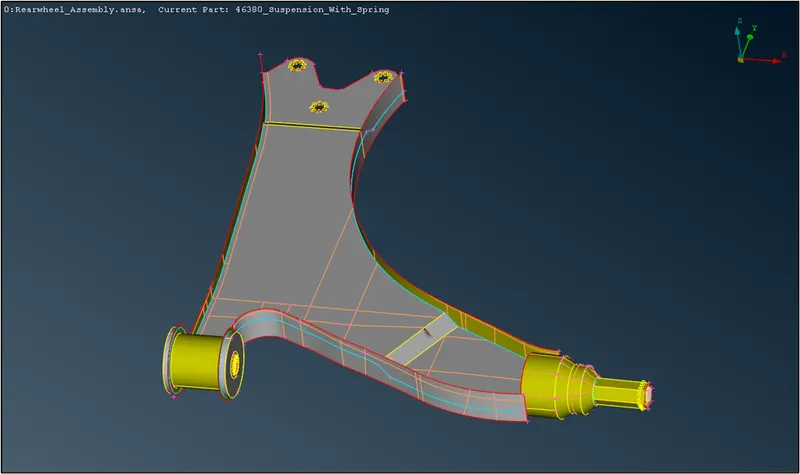
   Fig.4. Lower Control Arm Midsurface

4. Before generating the mesh on the midsurfaces, we have to feed the mesh criteria to the algorithm per criteria III.D so that we get the desired quality. For this, we click the Quality Criteria and input the required criteria. The Mesh Parameter is also changed where we set the average element length as 4 and the min and max length is set to 2 and 6 respectively.

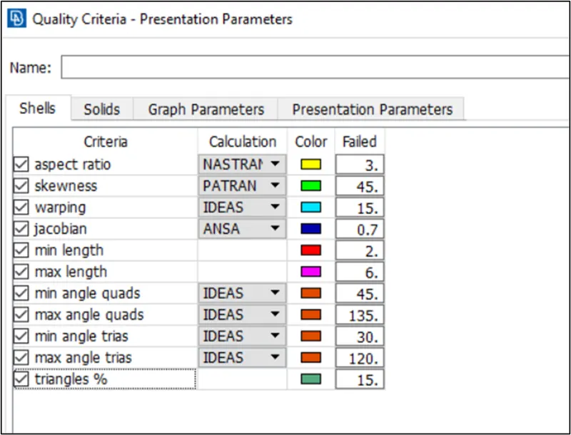
   Fig.5. Mesh Quality Criteria III.D.

5. To get a proper mesh flow, we have to start the mesh generation from the inside and move outwards. Also, the macros should be divided into parts so that the algorithm can generate a mesh with a good flow. To do this we use the Cut option for Macros in the Mesh tab.
6. While meshing the components, we will encounter the tria elements which will be inevitable. But some trias like back-to-back and opposite trias have to be avoided at all costs. We use the split option to remove such elements. A very good article has been made on this. The tria element is split till it reaches the nearest opposing tria. Once that is done, the trias can be joined to form Quads and then the mesh can be smoothened out.

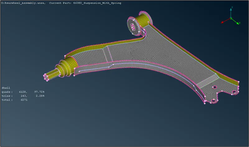
   Fig.6. Mesh on Lower Control Arm

7. Now it's a good practice to view the Quality of mesh while it is being created so that any discrepancy can be rectified easily before the whole part is meshed. Hence, the Hidden mode is switched on to see the failing elements. To rectify any failing elements, we have to play around with various options. In some cases, by using the Smooth option, the failing elements are rectified. But in other cases, we will have to make the mesh finer so that the major area is covered without abusing the criteria.
8. Since the mesh is assigned with the respective properties of the midsurfaces, the thickness is also defined to the mesh. This can be viewed by switching the Draw shell as a solid option.

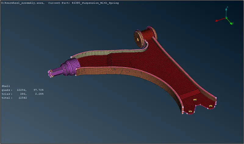
   Fig.7. Mesh Thickness display

9. The remaining components with similar traits are also meshed with a similar procedure.

B. 3D Tetra mesh generation for components with thickness more than 5mm:-

1. Before generating the mesh on the model, we have to feed the mesh criteria to the algorithm so that we get the desired quality. For this, we click the Quality Criteria and input the required criteria. The Mesh Parameter is also changed where we set the average element length as 4 and the min and max length is set to 2 and 6 respectively. Also, for Solid mesh, the only criteria used is Collapse with the value of 0.2.

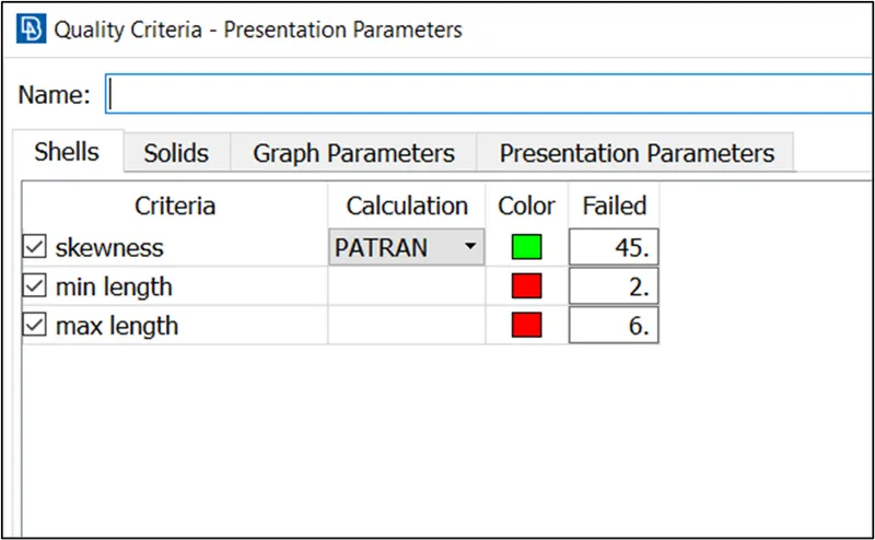
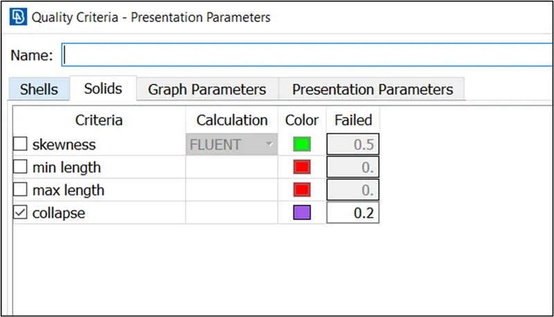
   Fig.8. Mesh Quality Criteria

2. Now the model is first meshed with shell mesh (tria and ortho tria) and then move on with solid mesh. For this, we navigate to Mesh Generation → Spot Mesh → Ortho Tria. It is ensured that the curved features and fillets are first meshed with ortho trias and then the rest of the flat surfaces are meshed with tria elements. Now the macro mesh is reconstructed for a better mesh flow and removes any discrepancy on its own.
   
3. After the ortho tria elements are generated, we shall create the trial shell mesh on the flat surfaces as seen below in figure 6. This way, we mesh the whole model with shell mesh.

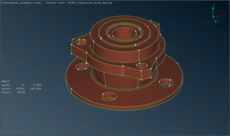
   Fig.9. Shell Mesh on the Hub Component

4. With the shell mesh in place, we can now move on to the volume/solid mesh for generating the tetra elements. To do this we will first have to navigate to Volume Mesh → Volume → Define → Detect on: Selected → Select the volume to be solid meshed. Since a volume mesh can be only applied to closed volumes, we shall note whether the shell meshed components form a closed volume or not.
5. Once selected, the volume will be defined by a new property with the card name as PSOLID in contrast to the previously used PSHELL. The Volume editor volume window will open and the status of the selected volume will be unmeshed. So, we right-click on the volume name and select edit. Here, we change the mesh type as Tetra FEM as the suitable algorithm. The selection is confirmed by pressing OK. Now, the volume is right-clicked again and the Remesh option is clicked. This will mesh the whole volume with tetra elements. This will be done for all the components.

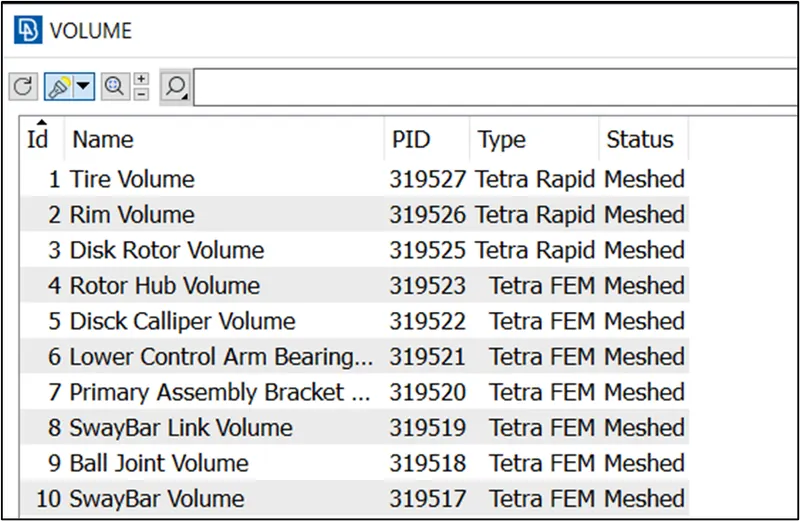
   Fig.10. Volume List with Algo type

6. Finally, the model should pass the Tet Collapse parameter. No element should fail for this parameter. To correct any failing element, we can conduct a trial and error using the MV Node option which can certainly clear the failing element. This is the best alternative since with this procedure we can avoid kinks or raised edges. Also, we can remove the 2D shell mesh since they provide no purpose in further analysis. With this, our procedure is completed.

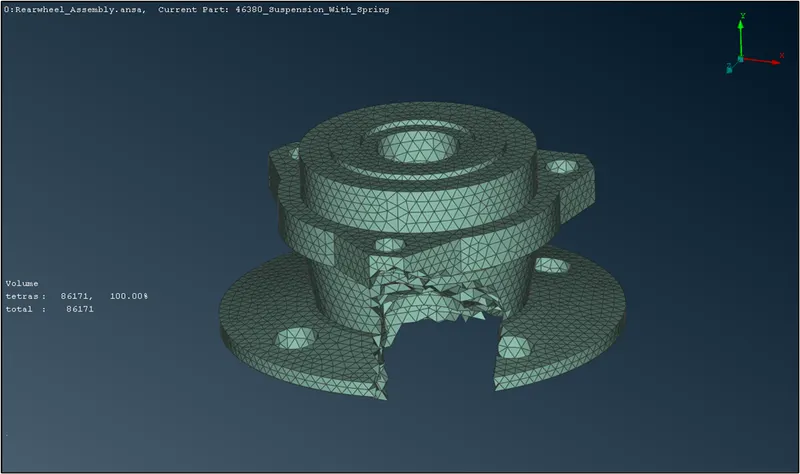
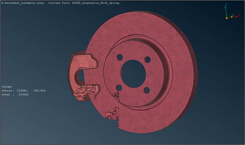
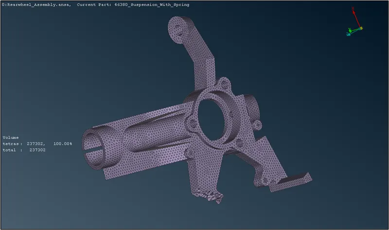
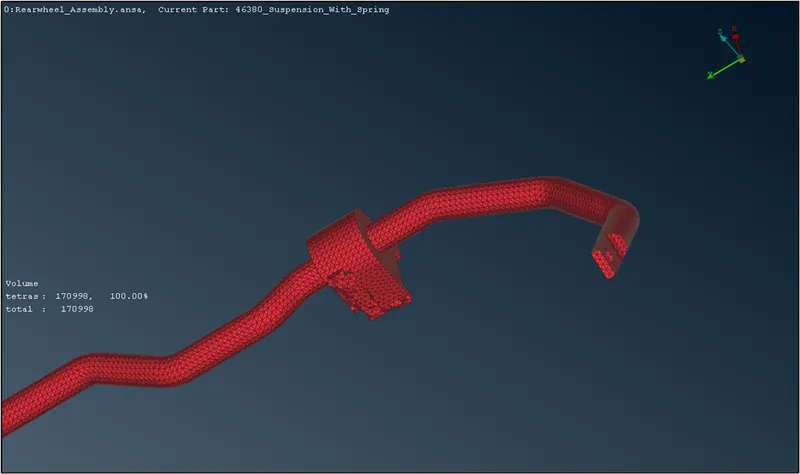
   Fig.11. Solid Meshed Components with cross-sections

7. In the case of the Tire and Rim components, the mesh criteria and parameters have to be changed as seen in figure 12. The Mesh Parameter is also changed where we set the average element length as 6.5 and the min and max length is set to 5 and 10 respectively. Also, for Solid mesh, the criteria used is Collapse which is left at a value of 0.2.

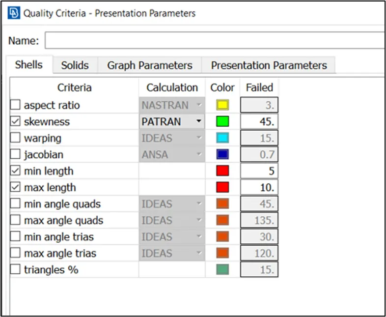
   Fig.12. Mesh Quality Criteria for Rim & Tire component

8. For tetra meshing of the tire and rim component, the same procedure is used as above. The following figure shows the result.

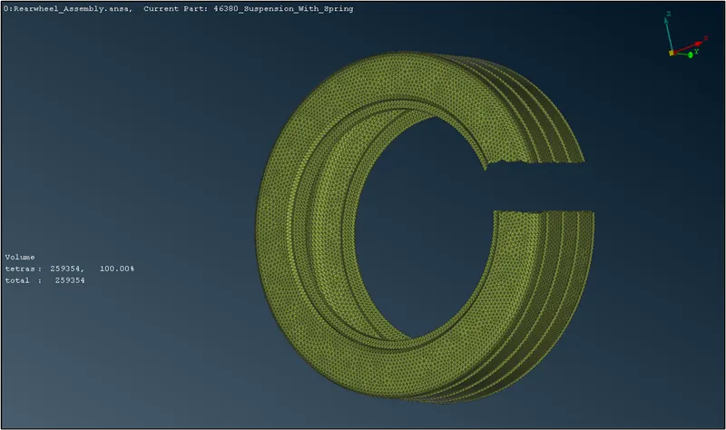
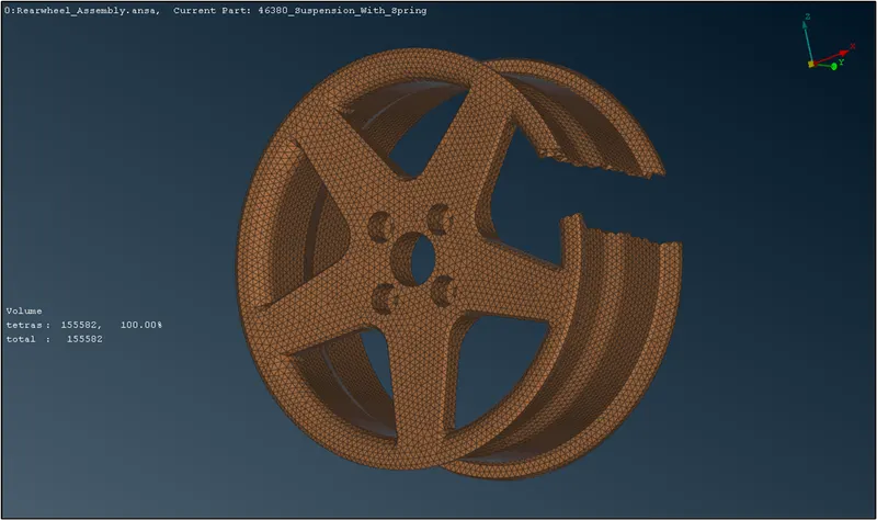
   Fig.13. Solid Mesh on Tire and Rim

9. During the meshing procedure of the rim, due to the complexity of the geometry, there exist some failing elements that cannot be corrected per the given quality criteria. These OFF elements can be neglected.

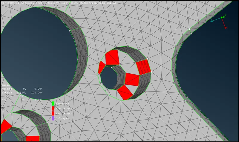
   Fig.14. Failing Elements on Rim component

C. 1D Element generation for Coil Spring Component:-

1. For the Coil Spring, 1D elements shall be generated for further analysis. First, a 3D curve is created at the middle of the spring cross-section using the Middle option from the Curves menu.

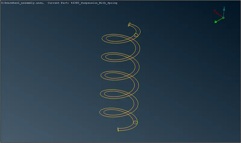
   Fig.15. Middle Curve creation

2. There is more than one curve formed and shall be converted to a single curve. The Connect option is used to do so. As a reference, a 3D point is created at the COG of the curve.

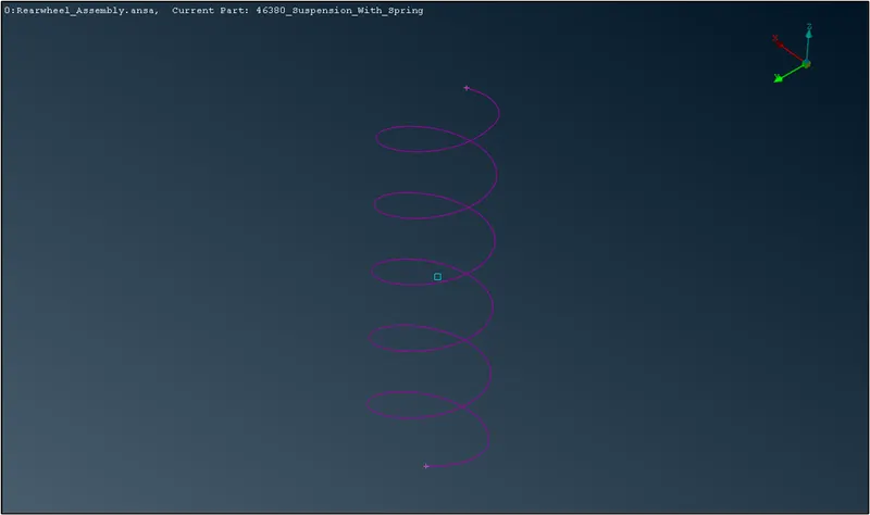
   Fig.16. Curve with COG point

3. Now, from the Nastran solver deck, the CBAR element option is selected. Then the option Orientation node is toggled ON and the curve is selected. For the node, the COG point is selected. For the element length, we put in a 3 mm value.
4. Next, the PID for the 1D elements has to be created by clicking on New. Then, by selecting the A box, the Shift + ? combination is used to direct to section parameters where the radius value is fed as 5 mm. The OK button is clicked twice. This will create our 1D elements for representing the Coil Spring.

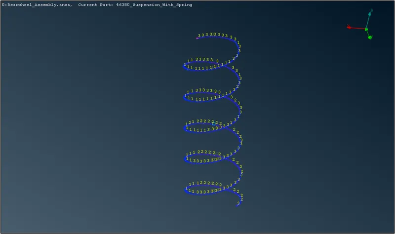
   Fig.17. 1D elements for Coil Spring

5. Finally, from the Parameters presentation sub-menu of the Quality criteria menu, the option "Line element representation" is switched ON and the draw mode is set to Solid. This finishes the modeling of the spring.

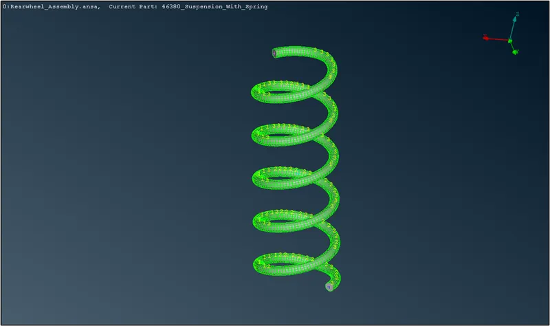
   Fig.18. 1D elements Solid representation

D. Creation of appropriate connections on the model:-

1. The Suspension model provided has a variety of components that require connections. Though no data about these connections is given, we shall use our best judgment to deploy the apt connections.
2. For a majority of components, RBE2 connectors can suffice. These are used to create rigid connections between the components. For this, we navigate to the NASTRAN deck → Elements → RBE2 → Many Nodes and select the nodes at the perimeter using the loop option, and click the middle mouse button.

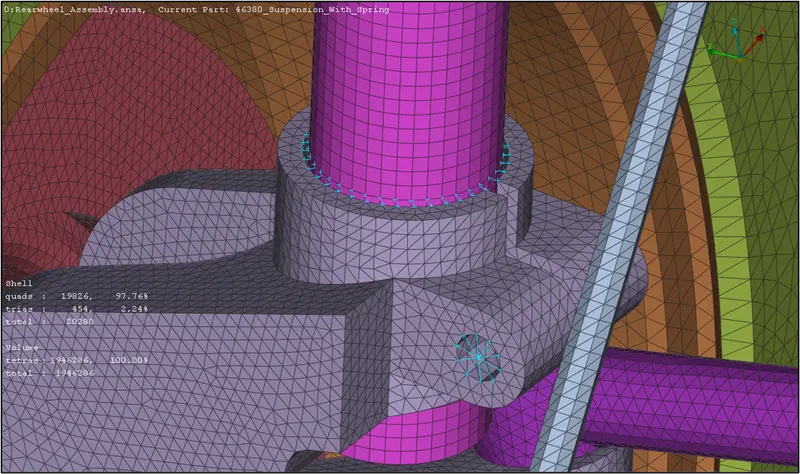
   Fig.19. RBE2 connection on Suspension Strut

3. There are cases where the DOF in some direction has to be unconstrained. The lower control arm is an example of this. The deployed connection has DOF constraint in only 5 directions and is unconstrained about X-axis.

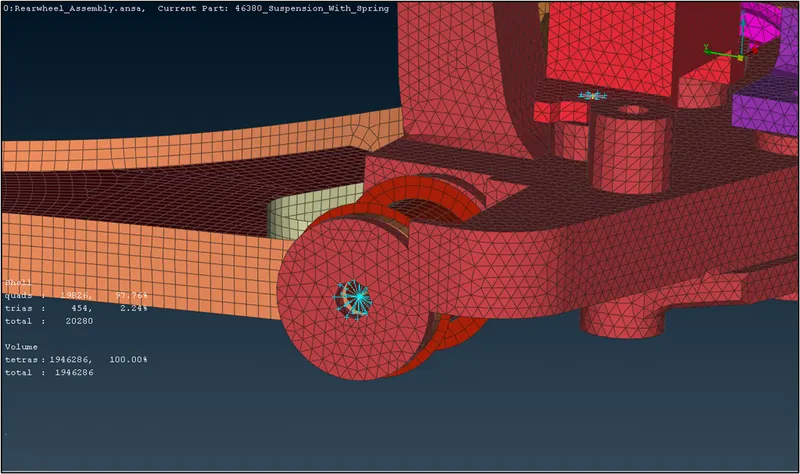
   Fig.20. RBE2 connection on Lower Control Arm

4. On the Rims and other components, bolt connections should be deployed. For this, we navigate to Topo → Points → On COG and create 3D points on the required places as seen below. Then we go to Assembly → Convert → 3D Points → Bolt and select the 3D points we had created.

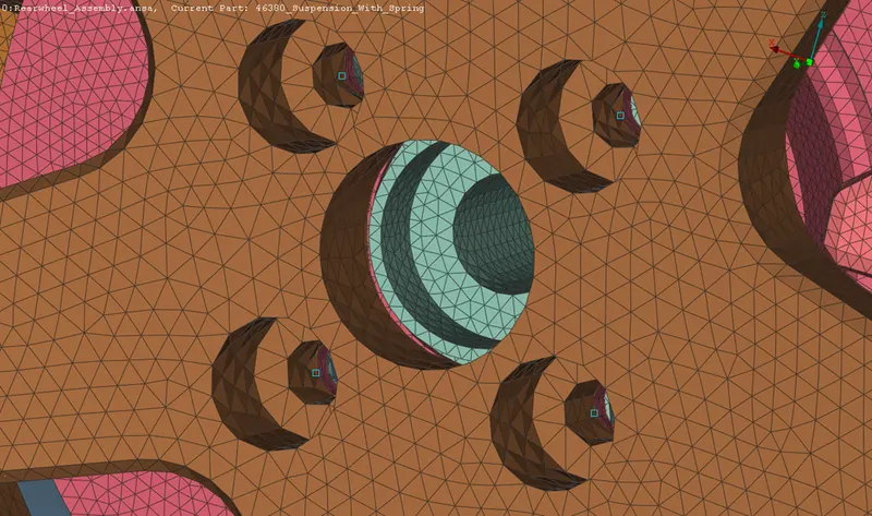
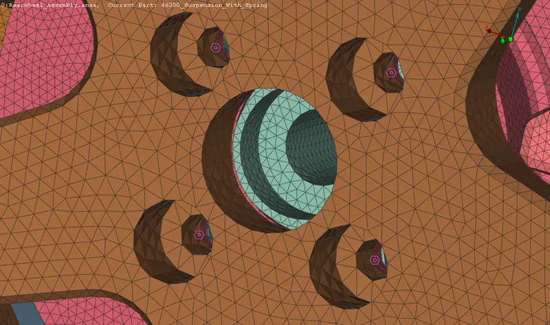
   Fig.21. 3D points to Connectors for Bolts

5. Next, with the help of the connections manager assistant, we shall select all these connections and make adequate changes in the manager menu. In which some parameters such as PID 1, PID 2, FE representation type should be selected. Then by selecting Apply, Realize the connection will be realized.

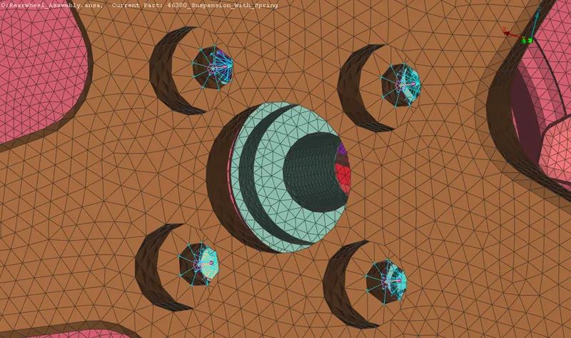
   Fig.22. Creation of the Bolt Connections

6. The parts that are aligned parallel or perpendicular can be connected with SeamWeld connections with either Overlap Shell or Y-Joint Shell. To create the Seamweld, a curve has to be created. This is done by navigating to Mesh → Perimeters → Feat2Curv. The curve is then converted into a Seam Line. Assembly → Convert → Curves → Seam Line.

7. Now, the connection manager is opened and the Seam Line is selected. The parts to be joined are selected under P1 and P2. Since the parts to be joined are parallel to each other, the FE Rep Type selected is 'OVERLAP SHELL, and the properties are defined. If the parts to be joined are perpendicular to each other then, Overlap-SHELL is selected as the FE Rep Type.

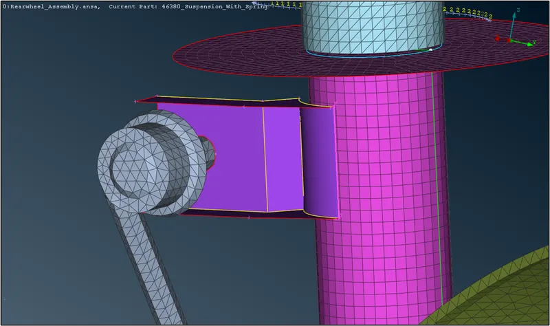
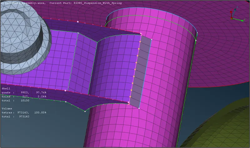
   Fig.23. SeamWeld Connection realized

8. Finally, with the interface of Tire and Rim, the connection should be CBUSH since their connection is elastic due to the rubber composition of the Tire. So to represent that, the CBUSH elements have to be used since it behaves as an elastic in all three directions.
9. Initially, the curves are needed to provide a reference for the connectors. For that, the Feat2Curv option in the perimeters from the topo module is used. And the FEA edges are selected one by one and then it is converted into curves, which are represented by purple-colored lines at the edges. It is made sure that two adjacent curves are selected to create the seam line. Then these curves are converted into "spot line".

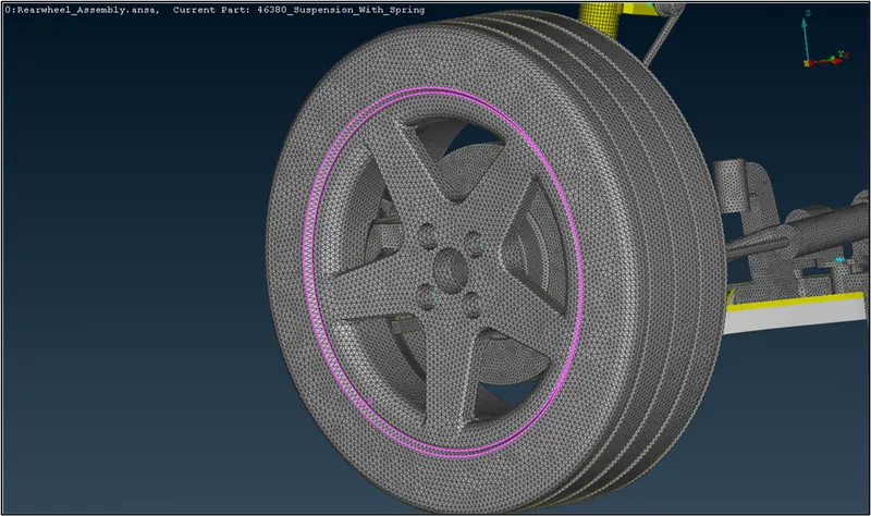
   Fig.24. SpotLine for CBUSH

10. Now, these spot lines are realized by selecting the line by line and specifying the parameters such as spacing between the CBUSH elements, specifying PARTI & PART 2, specifying FE representation type as RBE3-CBUSH-RBE3, and assigning RBE3 pin flags(DOF) in all directions.
11. A new PID should be created, which is done by selecting Shift+? from the keyboard by placing the cursor in the PBUSH ID row. After selecting a New option, a dialog box appears as shown in figure 14, which represents PID for the CBUSH elements. In that, the 6 stiffness values are entered, which are pre-calculated. For K1, K2, K3 the value is set to 0.001 and 10 for the rest.

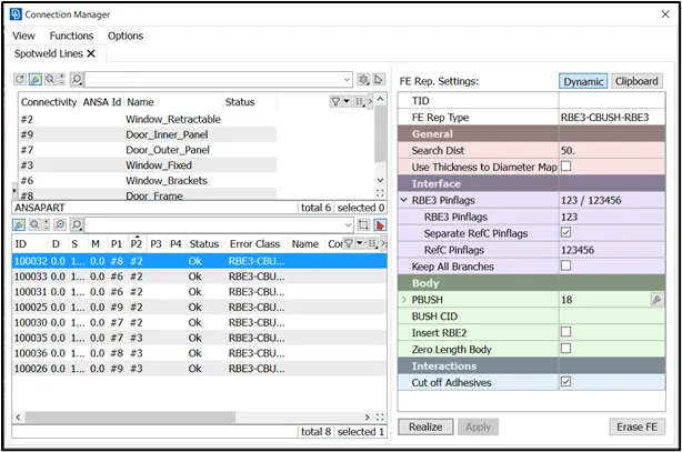
    Fig.25. Connection Manager for CBUSH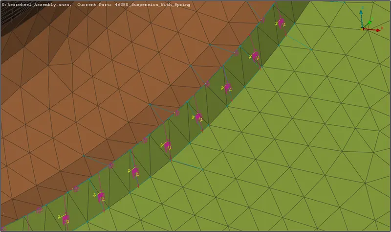

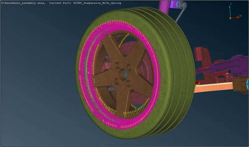
    Fig.26. Final Realized CBUSH Connectors

E. Symmetry command to reflect the half-finished model to the other side:-

1. After performing the quality optimization of all components and connectors deployment, the resultant model is mirrored about its respective symmetry.
2. For this, the Transform command is used from the utility tab. The required elements are selected and then the Mirror 3 points plane option is selected. The mandatory nodes are selected for the symmetry and the mesh will be transformed.

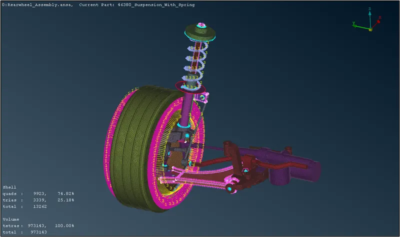
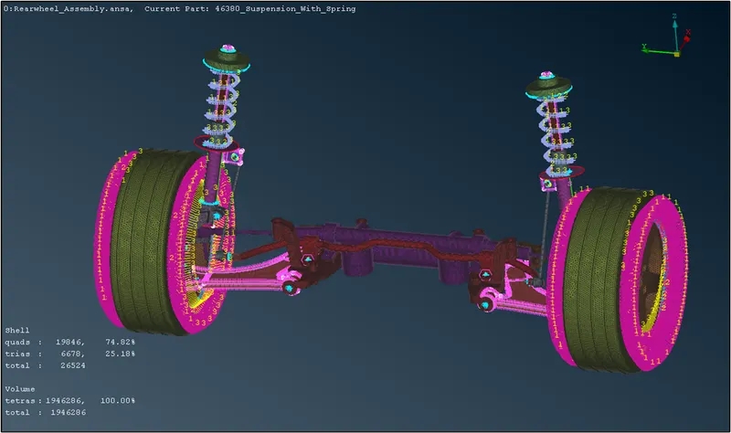
   Fig.27. Symmetry Transformation

3. With this, the procedure for Project 2 comes to an end.

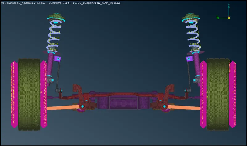
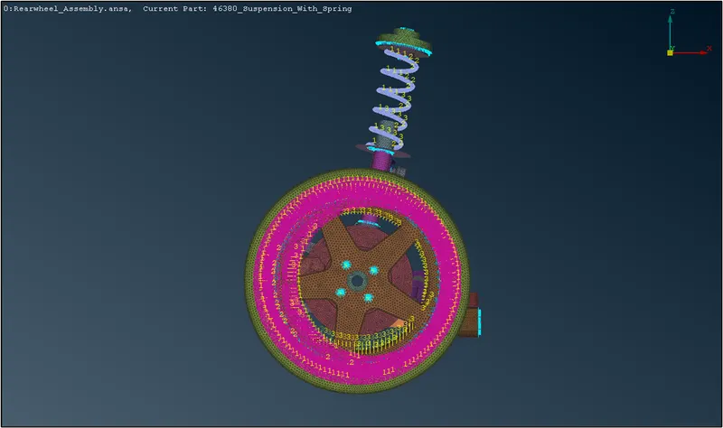
V. RESULTS - FINAL FE MODEL

VI. LEARNING OUTCOMES

• From the above assignment, the following points were learned in ANSA software:-

1. 2D Shell and 3D Solid Mesh generation techniques were perfected.
2. Mesh Quality and Parameters check
3. Creation of diverse kinds of connectors with different IDs.
4. Debugging of unrealized connectors.

VII. CONCLUSIONS

• The FE modeling of the given Rear View Mirror assembly has been completed and the following points are drawn as conclusions: -

1. With this challenge, the methods of tetra meshing were successfully learned.
2. All the given components in the model were meshed with 3D Tetra elements using suitable methods.
3. All the meshed components were ensured to pass the element quality criteria.
4. All the Connectors were efficaciously created and deployed according to the given connection details.
5. The mesh of the whole assembly was rectified after deploying the connectors and was thoroughly ensured to pass all the qualifying mesh parameters.