FILE PARSING OF NASA'S THERMODYNAMIC DATA USING MATLAB

I. OBJECTIVES

1. To write a program that can parse the NASA Thermodynamic Data and extract the 14 coefficients and calculates the enthalpy, entropy, and specific heats for all the species in the data file.
2. To calculate the molecular weight of each species and display it in the command window.
3. To plot the Specific Heat, Enthalpy, and Entropy for the local temperature range (low temperature: high temperature) unique for each species.
4. To save the plots as images with appropriate names and dump them in separate folders for each species with suitable names.
5. To display the saved folders of each species and the plots for O2, CO2, and N2 in the report.

II. INTRODUCTION

1. File Parsing: - Parsing, syntax analysis, or syntactic analysis is the process of analyzing a string of symbols, either in natural language, computer language, or data structures, conforming to the rules of a formal grammar. So simply, Parsing a file basically means reading in a data stream of some sort and building an in-memory model of the semantic content of that data. This aims at facilitating performing some kind of transformation on the data.

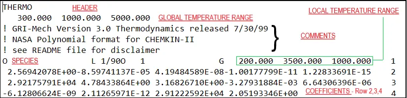
2. NASA's Thermodynamic Data File: - NASA came up with polynomials that can be used to evaluate thermodynamic properties such as Specific Heat, Enthalpy, and Entropy. They have also documented the coefficients that are required to evaluate these polynomials for 1000+ species. This file is provided in a '.dat' the file format which can be opened using the Notepad for accessing the species-wise properties. 'THERMO.dat' file is a data file containing 14 coefficients for 53 different species given by NASA. These coefficients are utilized to calculate the specific heat, enthalpy, and entropy for a particular element. Each element has its own range of local temperatures. Below we can see the layout of the THERMO.dat file as opened in the notepad.

3. Thermodynamic Properties: - Following are the thermodynamic properties that were evaluated for this report.

1. Specific Heat, Cp [KJ/Kg-K] - the ratio of the quantity of heat required to raise the temperature of a body one degree to that required to raise the temperature of an equal mass of water one degree. Formulae associated; High Temperature Range - `frac{Cp}{R}= a1+a2*T+ a3*T^2+a4*T^3+a5*T^4` Low Temperature Range - `frac{Cp}{R}= a8+a9*T+ a10*T^2+a11*T^3+a12*T^4`
2. Enthalpy, H [KJ/Kg] - The sum of the internal energy and the product of the pressure and volume of a thermodynamic process. Enthalpy is an energy-like property or state function—it has the dimensions of energy (and is thus measured in units of joules or ergs), and its value is determined entirely by the temperature, pressure, and composition of the system and not by its history. Formulae associated; High-Temperature Range - `H/(RT) = a1 + a2*T/2 + a3*T^2/3 + a4*T^3/4 + a5*T^4/5 + a6*1/T` Low-Temperature Range - `H/(RT) = a8 + a9*T/2 + a10*T^2/3 + a11*T^3/4 + a12*T^4/5 + a13*1/T`
3. Entropy, S [KJ/Kg-K] - It is the measure of a system’s thermal energy per unit temperature that is unavailable for doing useful work. Because work is obtained from ordered molecular motion, the amount of entropy is also a measure of the molecular disorder, or randomness, of a system. Formulae associated; High-Temperature Range - `frac{S}{R}= a1*lnT+a2*T+a3*frac{T^2}{2}+ a4*frac{T^3}{3}+a5*frac{T^4}{4}+a7` Low-Temperature Range - `frac{S}{R}= a8*lnT+a9*T+a10*frac{T^2}{2}+ a11*frac{T^3}{3}+a12*frac{T^4}{4}+a14`

III. MATLAB PROGRAM

A. Program to Parse NASA's Thermodynamic Data

% A program to perform File Parsing of NASA Thermodynamic Data

clear all
close all
clc

% Loading the file
Thermo = fopen('THERMO.dat','r'); % Opening in Read mode

%% Line by Line reading
% LINE #1
tline1 = fgetl(Thermo); % Skipped Header

% LINE #2
tline2 = fgetl(Thermo);
GlobalTemp = strsplit(tline2,' '); % Strings split by space
Low_GlobalTemp  = str2num(GlobalTemp{2});
Mid_GlobalTemp  = str2num(GlobalTemp{3});
High_GlobalTemp = str2num(GlobalTemp{4});

% LINES #3,4,5
for i = 1:3
     fgetl(Thermo); %Skipped
end 

%% Loop Initiation for Individual Species Data Evaluation
for i = 1:53
    
    Line_1 = fgetl(Thermo);
    
    Species_Prop = strsplit(Line_1,' ');
    Species_Name = (Species_Prop{1});
    Length = length(Species_Prop);
    
    % Extracting Species Name and Local Temperature Range
    Low_LocalTemp  = str2num(Species_Prop{Length-3});
    Mid_LocalTemp  = str2num(Species_Prop{Length-1});
    High_LocalTemp = str2num(Species_Prop{Length-2});
    
    % Extracting Coefficients
    Line_2 = fgetl(Thermo);
    
    a   = findstr(Line_2,'E');
    a1  = str2num(Line_2(1:a(1)+3));
    a2  = str2num(Line_2(a(1)+4:a(2)+3));
    a3  = str2num(Line_2(a(2)+4:a(3)+3));
    a4  = str2num(Line_2(a(3)+4:a(4)+3));
    a5  = str2num(Line_2(a(4)+4:a(5)+3));
    
    Line_3 = fgetl(Thermo);
    
    b   = findstr(Line_3,'E');
    a6  = str2num(Line_3(1:b(1)+3));
    a7  = str2num(Line_3(b(1)+4:b(2)+3));
    a8  = str2num(Line_3(b(2)+4:b(3)+3));
    a9  = str2num(Line_3(b(3)+4:b(4)+3));
    a10 = str2num(Line_3(b(4)+4:b(5)+3));
    
    Line_4 = fgetl(Thermo);
    
    c   = findstr(Line_4,'E');
    a11 = str2num(Line_4(1:c(1)+3));
    a12 = str2num(Line_4(c(1)+4:c(2)+3));
    a13 = str2num(Line_4(c(2)+4:c(3)+3));
    a14 = str2num(Line_4(c(3)+4:c(4)+3));
    
    % Molecular Weight Evaluation
   Element = ['H','C','N','O','S','A'];
   Weight  = [1 12 14 16 32 40];
   Mol_Weight = 0;
    for i = 1:length(Species_Name)
        for j = 1:length(Element)
            if strcmpi(Species_Name(i),Element(j))
                Mol_Weight = Mol_Weight + Weight(j);
                l = j;
            end
        end
        n = str2num(Species_Name(i));
            if n > 1
                Mol_Weight = Mol_Weight + Weight(l)*(n-1);
            end
    end
    
    % Displaying the values 
    fprintf('n Molecular Weight of %s = %f Units',Species_Name,Mol_Weight)
    disp(' ')
    
    % Input Values for Thermodynamic Parameters
    R = 8.314; % Universal Gas Constant
    T = linspace(Low_LocalTemp,High_LocalTemp,500); % Local Temperature Range
    
    % Thermodynamic Parameters Evaluation
    for j = 1:length(T)
        if T(j) > Mid_LocalTemp
            Cp = (a1+a2.*T+a3.*T.^2+a4.*T.^3+a5.*T.^4).*R;
            H  = (a1+(a2.*T)./2+(a3.*T.^2)/3+(a4.*T.^3)/4+(a5.*T.^4/5)+a6./T).*T.*R;
            S  = (a1*log(T)+a2.*T+(a3.*T.^2)/2+(a4.*T.^3)/3+(a5.*T.^4)/4+a7).*R;
        else
            Cp = (a8+a9.*T+a10.*T.^2+a11.*T.^3+a12.*T.^4).*R;
            H  = (a8+(a9.*T)/2+(a10.*T.^2)/3+(a11.*T.^3)/4+(a12.*T.^4/5)+a13./T).*T.*R;
            S  = (a8.*log(T)+a9.*T+(a10.*T.^2)/2+(a11.*T.^3)/3+(a12.*T.^4)/4+a14).*R;
        end
    end 
        
    % Folder Creation
    mkdir(Species_Name)
    cd(Species_Name)
    
    % Plot Commands
    % Plot#1 TEMPERATURE vs SPECIFIC HEAT
    figure(1);
    plot(T,Cp,'linewidth',2,'color','b')
    xlabel('Temperature[K]')
    ylabel('Specific Heat[KJ/Kg-K]')
    title(sprintf('Temperature vs Specific Heat plot for %s',Species_Name))
    grid on
    saveas(figure(1),'Specific Heat.jpg')
    
    % Plot#2 TEMPERATURE vs ENTHALPY
    figure(2);
    plot(T,H,'linewidth',2,'color','r')
    xlabel('Temperature[K]')
    ylabel('Enthalpy[KJ/Kg]')
    title(sprintf('Temperature vs Enthalpy plot for %s',Species_Name))
    grid on
    saveas(figure(2),'Enthalpy.jpg')
    
    % Plot#3 TEMPERATURE vs ENTROPY
    figure(3);
    plot(T,S,'linewidth',2,'color','g')
    xlabel('Temperature[K]')
    ylabel('Entropy[KJ/Kg-K]')
    title(sprintf('Temperature vs Entropy plot for %s',Species_Name))
    grid on
    saveas(figure(3),'Entropy.jpg')
    
    cd(pwd)
    cd ..
end
%%
fclose(Thermo); % THERMO.dat file closed

A.1. Steps for the above program: -

1. The program is commenced with the basic 'clear all','close all','clc' commands.
2. In order to open the file, the 'fopen' command is used, 'THERMO.dat' is the file name and 'r' relates to reading a file. This is saved as a variable for further reference.
3. From this step, the process of Line reading is started. The 'fgetl' command is used for this purpose. The variable that was saved is now used for reading the line from that .dat file.
4. Line number two consists of the Global Temperature range. For extracting the values, we use the split tactic where we identify a delimiter that acts as a reference point. We initiate this by using the 'strsplit' command. For our case, ' ' (literally space mark) is the delimiter where either side of the space hosts the temperature value. Since we can identify on which position the values lie with respect to space, the string values are converted to number characters using 'str2num'.
5. 53 species data given in the file, we initiate a loop that follows the length of the number of species. Taking this step will repeat all the below-mentioned processes 53 times.
6. The first line of the species data is read similarly to Step 3. The line is split similar to that of Step 4. Thus, the name of the species is extracted as the first string. The length of this line is saved as a variable.
7. The Local Temperature range lies before one string at the end of this line. Hence, we use 'st2num' to extract all three temperature values using the code seen above.
8. Further, three more lines have to be read that contain or 14 coefficients. All these have been extracted by the strategy as seen in the program above.
9. In order to find the Molecular Weight of each species, the basic Elements, and their respective Atomic weights have to be fed in the code for evaluation. This is done using the symbols of the elements and saving them in an array. The respective atomic weights are saved accordingly.
10. A 'for' loop is initiated for the length of the Species Name. Another 'for' loop is initiated within for the length of the Element array. Under these loops, a command known as 'strcmpi' is used in order to compare the strings that are case sensitive. If the strings agree with the code, the value returned is true and it is added with the molecular weight of that very element. The technique can be understood by looking at the code itself.
11. The values of respective molecular weights are displayed on the command window.
12. A new 'for' loop is initiated for calculating the thermodynamic properties. Since we have to calculate for lower and higher temperature ranges, we use the 'if-else' loop that keeps the properties discrete for every species. This depends on the mid-range temperature that has been provided in the 'THERMO.dat' file. The formulae are fed accordingly.
13. A new folder is created using the 'mkdir' command so that the automatically created folders for the species are saved in one place. The 'cd' command is used for changing the current directory.
14. Basic plot commands are further given for comparison between all three thermodynamic properties and the temperature range. All plots are saved to the directory using the 'saveas' command.
15. The directory is converted back to the current one and the master loop is finally ended. The .dat file is also closed.

A.2. Results from the above program: -

1. Molecular Weights displayed in the Command Window

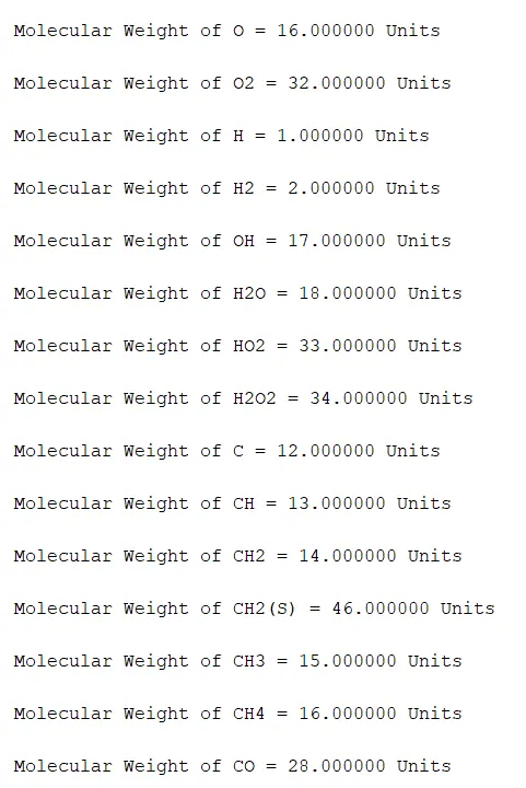
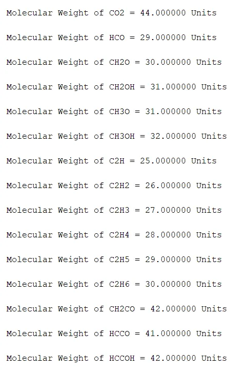
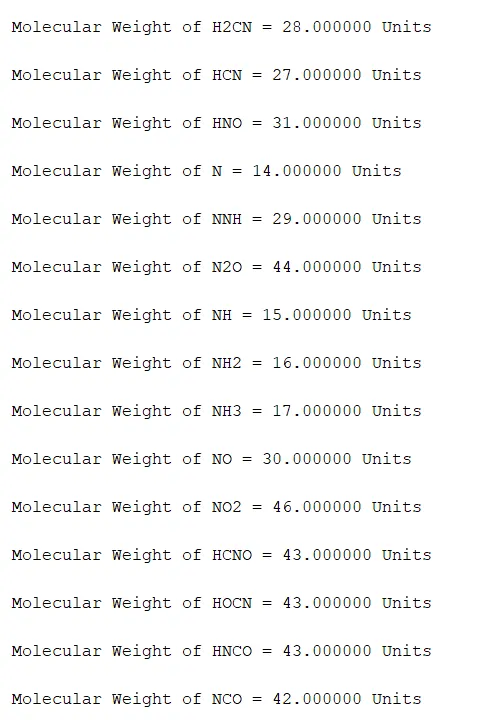
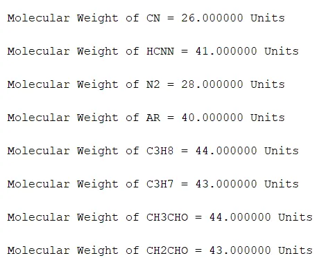
• The above screenshots show the values of Molecular Weights of every Species present in the file. This is as a result of running step 11. All Molecular weights are in standard units with approximated values.

2. Individual folders created for every Species

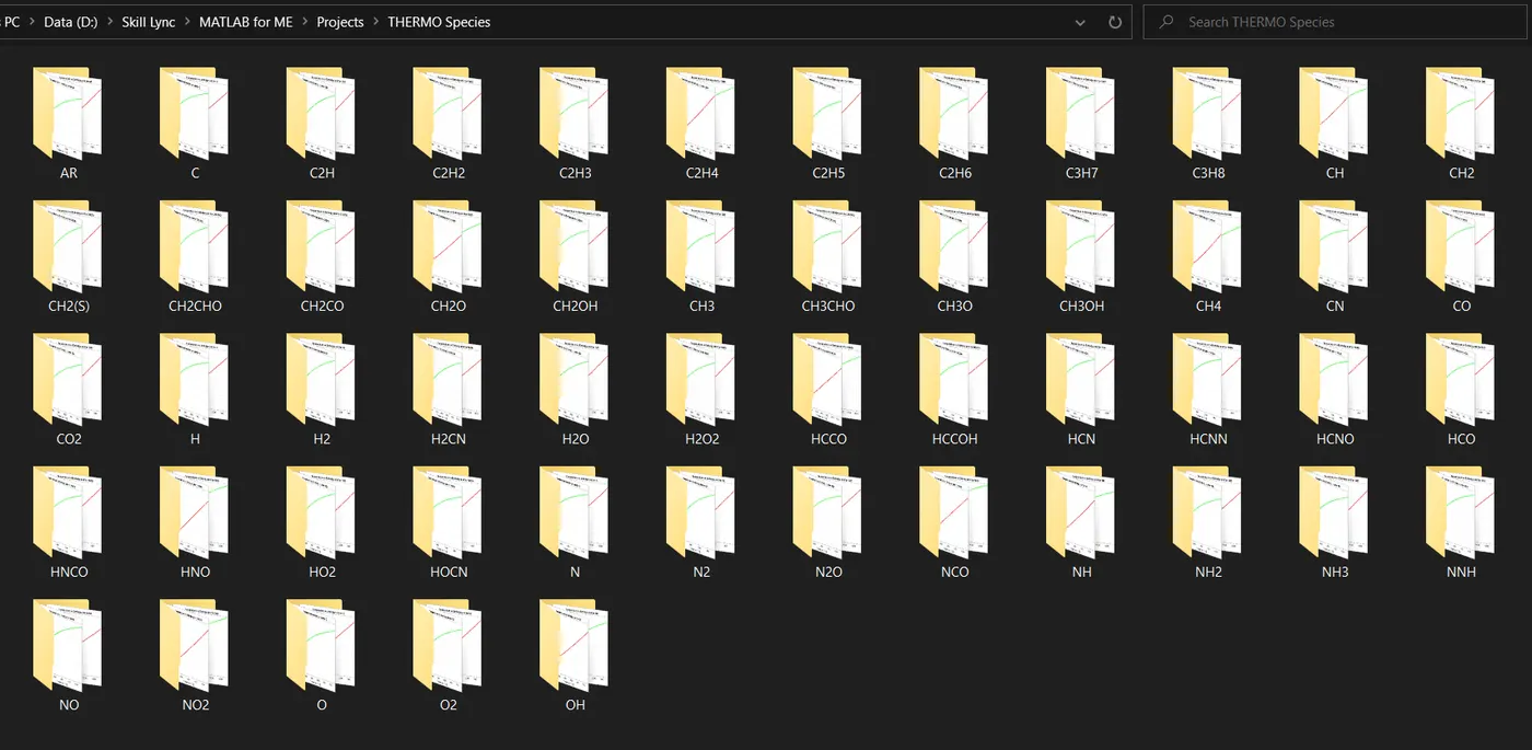
• The above screenshot shows the folders that were created by MATLAB and were saved here. This is a result of running step 13. This step makes it much more manageable and we can easily handle a large number of plots.

3. Plots created for every Species

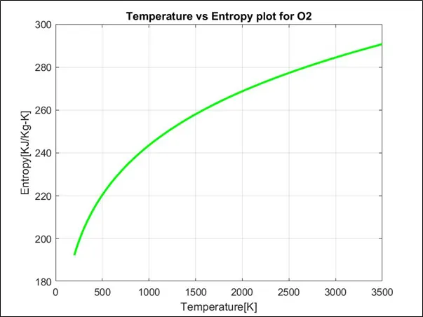
1. O2 Plots

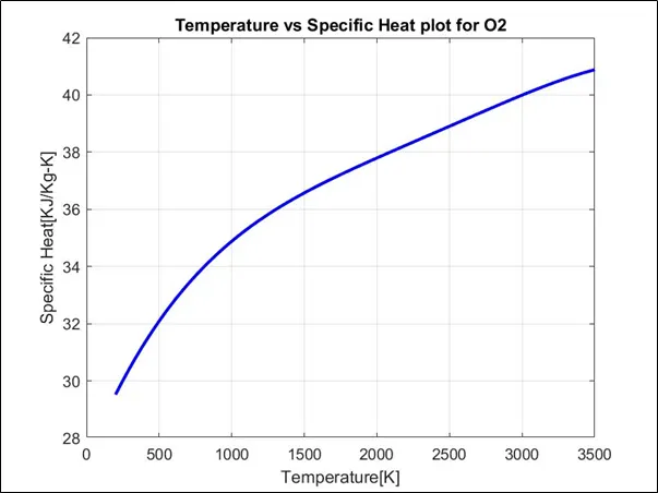
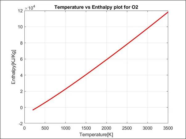
ii. N2 Plots

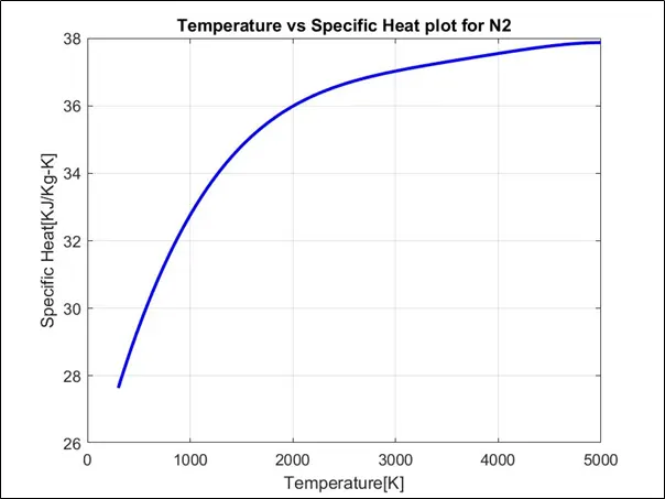
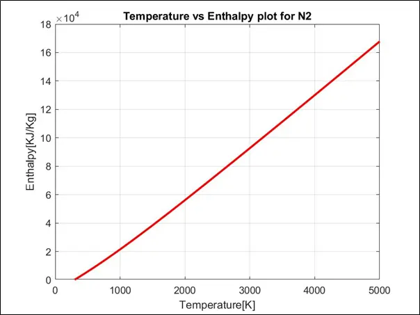
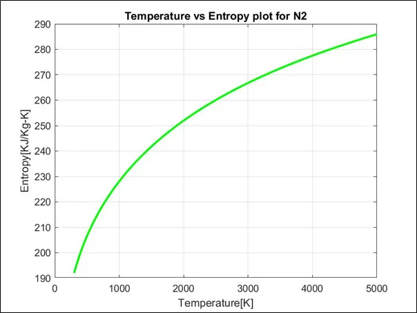
iii. CO2 Plots

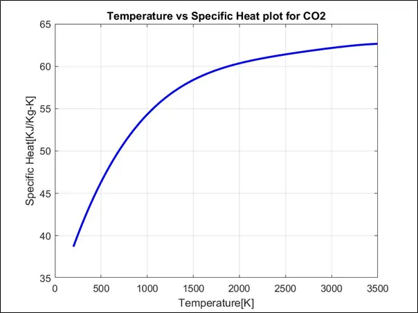
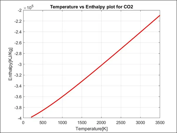
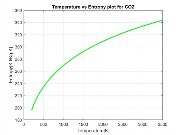
• The above plots represented by points i, ii, and iii show the variations of Specific Heat, Enthalpy, and Entropy with respect to the Temperature changes respectively. It can be easily observed that the thermodynamic properties do not stay constant as the temperature changes. Since this report discusses the use of File Parsing, we ignore the in-depth discussion of the above results.

A.3. Errors from the above program: -

Error #1 - Use of Incorrect brackets while using 'str2num' command

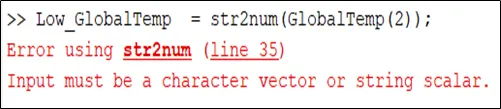
• The aforementioned error was encountered when the position of the 'cell' array was fed using the wrong type of parenthesis. The line which was read for this operation consists of different data types. These data types are save in a cell.
• A cell array is a data type with indexed data containers called cells, where each cell can contain any type of data. Cell arrays commonly contain either list of text, combinations of text and numbers, or numeric arrays of different sizes. We can refer to sets of cells by enclosing indices in smooth parentheses, (). In order to access the contents of cells by indexing, it is mandatory to use curly braces, {}.

No other intricate errors were delivered while programming.

IV. CONCLUSIONS

In this project report, the theory and application of the File Parsing were discussed for reading the 'THERMO.dat' file in MATLAB. Therefore, the following are the conclusions that can be made on the basis of the study done on the topic: -

1. The use of File Parsing in this report shows that we can read all kinds of desired data from files that contain them and utilize these data for any analysis that has to be done.
2. We can read data from any line, at any position in the file as long as we use the correct strategy to extract the same.
3. By using File Parsing, we can analyze any data file with good efficiency as well as save valuable time while doing so.

V. REFERENCES

• Concepts

1. Parsing - Wikipedia
2. NASA Polynomials - UC Berkeley
3. Specific Heat - Britannica
4. Enthalpy - Britannica
5. Entropy - Britannica

• Important MATLAB Commands

1. fopen - MathWorks
2. fgetl - MathWorks
3. strsplit - MathWorks
4. str2num - MathWorks
5. strcmpi - MathWorks
6. mkdir - MathWorks
7. if-elseif-else - MathWorks
8. cd - MathWorks
9. saveas - MathWorks