Project 2
The initialization script is run to load up the variables in the workspace.
The script is given below-
%% Vehicle Parameters
M = 1500; % Vehicle weight [kg]
Cr = 0.015; % Rolling resistance coefficient
Rw = 0.35; % Rolling radius [m]
Cd = 0.33; % Drag coefficient
Af = 2; % Frontal area [m2]
rhoa = 1.225; % Air density [kg/m3]
Vwind = 0; % Wind velocity [kmph]
g = 9.81; % Gravitational acceleration [m/s2]
theta = 0; % Slope [deg]
myu_road_tire = 1; % Coefficient of friction between tire - road interface
%% Powertrain Parameters
FDR = 3.73; % Final Drive Ratio / Diff Ratio
DiffEff = 0.99; % Differential efficiency (assumed independent of operating conditions)
NumGear = 4; % Number of gears in transmission
TransGear = [1:NumGear]; % Transmission Gears
TransRatio = [3.06, 1.62, 1, 0.7]; % Corresponding Transmission ratios
TransEff = 0.90; % Transmission efficiency (assumed independent of operating conditions)
TC_SR = [0, .5, .6, .7, .8, .87, .92, .94, .96, .97, 1]; % Torque Converter Speed Ratio (Matlab default) -> TurbSpd/PumpSpd
TC_TR = [2.232, 1.5462, 1.4058, 1.2746, 1.1528, 1.0732, 1.0192, 1, 1, 1, 1]; % Torque Converter Torque Ratio (Matlab default) -> TurbTrq/PumpTrq
TC_Cf = 1e-4 * [.72558, .66322, .63463, .59042, .51331, .4144, .29287, .22444, .12186, .04386, 0]; % Torque Converter Capacity Factor (Matlab default) -> PumpTrq/PumpSpd^2 [Nm/rpm^2]
load Vehicle_Data/Engine_data_1_9L_Saturn_95kW
load Vehicle_Data/Trans_Shift_map
load Vehicle_Data/EM_Honda_Insight_10kW
load Vehicle_Data/ESS_NiMH6
load Pack_Current_test.mat
ESS_init_soc = 0.8;
ESS_soc_max = 0.9;
ESS_soc_min = 0.6;
%% Driver Parameters
Kp = 10; % P gain for driver PI model
Ki = 1; % I gain for driver PI model
Drive_Cycle_Select = 1 ; % Drive cycle selection
% Drive cycle values in m/s
if Drive_Cycle_Select == 1
load DriveCycles/UDDS;
elseif Drive_Cycle_Select == 2
load DriveCycles/HWFET;
elseif Drive_Cycle_Select == 3
load DriveCycles/FTP;
elseif Drive_Cycle_Select == 4
load DriveCycles/US06;
elseif Drive_Cycle_Select == 5
load DriveCycles/NEDC;
elseif Drive_Cycle_Select == 6
load DriveCycles/WLTP;
end
time_end = cyc_time(end);
vel_end = cyc_vel(end);
The simulink model of the conventional vehicle is created ,it references the variables in the workspace.
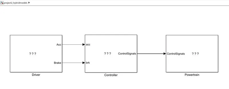
CONTROLLER BLOCK
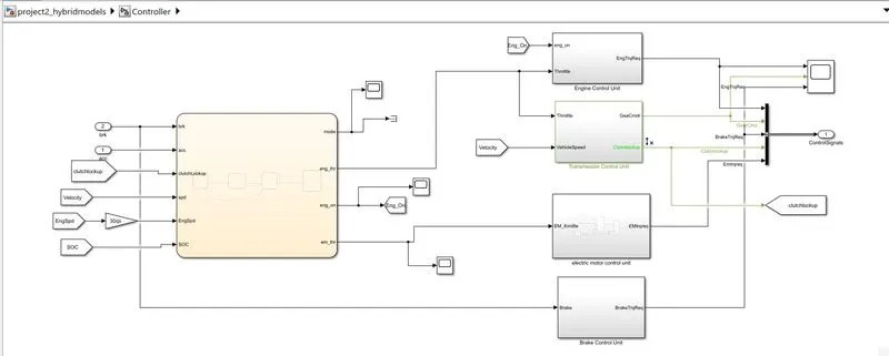
CHART INSIDE CONTROLLER BLOCK
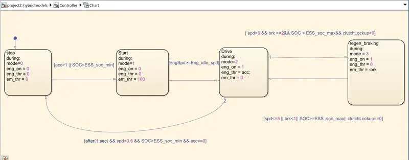
TRANSMISSION CONTROL UNIT
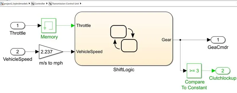
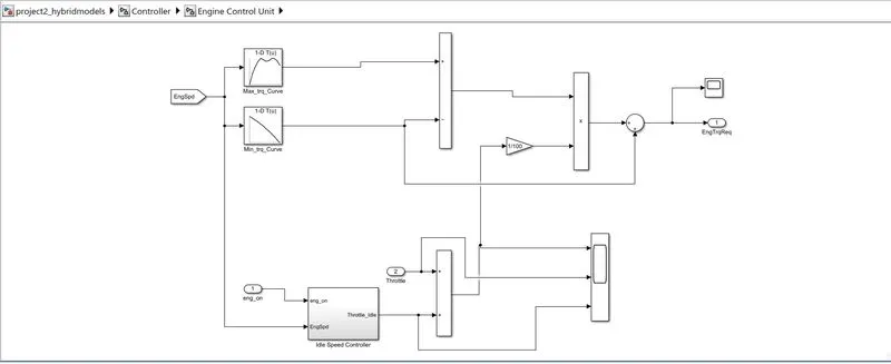
ENGINE CONTROL UNIT
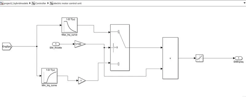
ELECTRIC MOTOR CONTROL UNIT
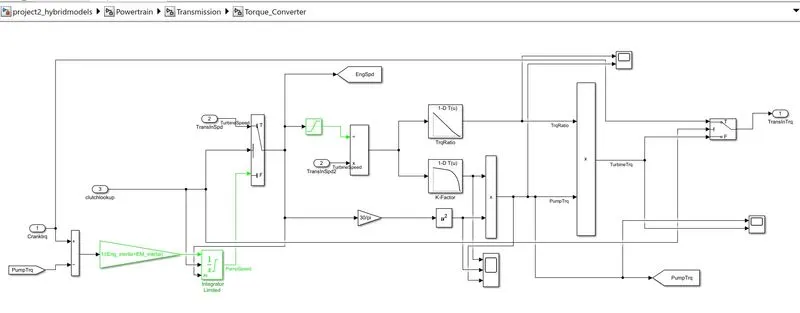
TORQUE CONVERTER BLOCK
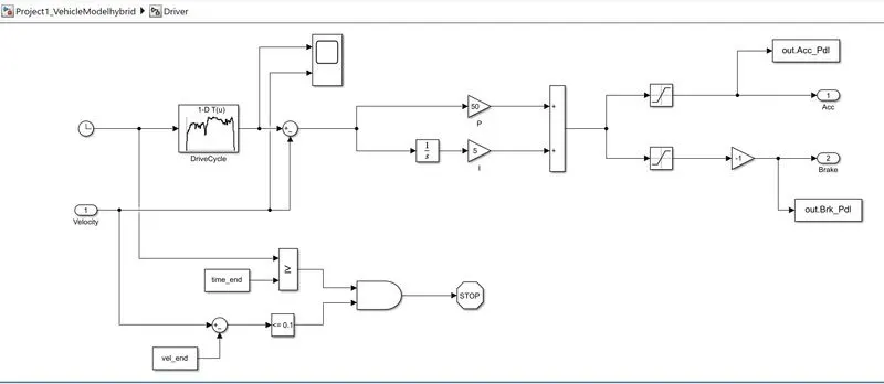
DRIVER BLOCK
POWERTRAIN BLOCK
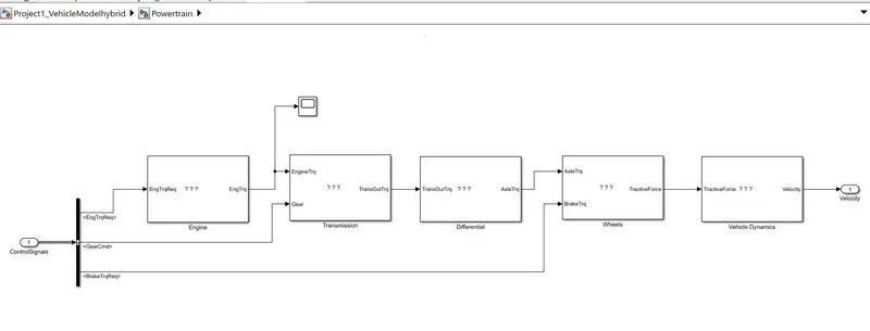
ENGINE BLOCK
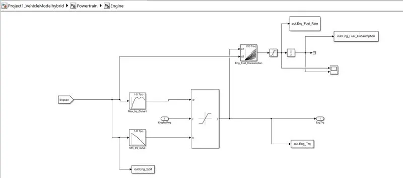
ELECTRIC MOTOR BLOCK
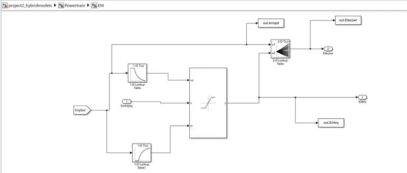
BATTERY BLOCK-
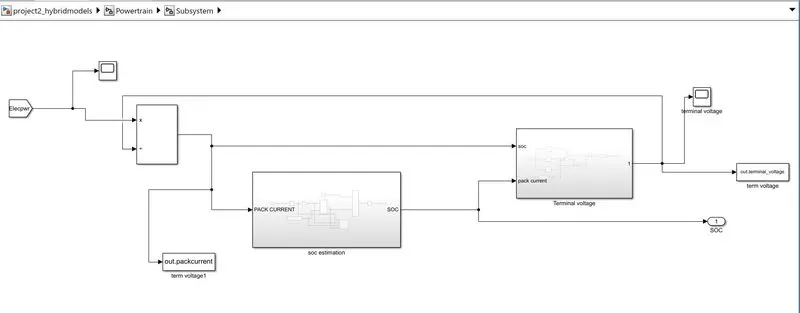
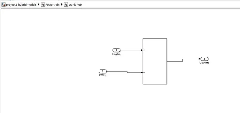
CRANKHUB BLOCK-
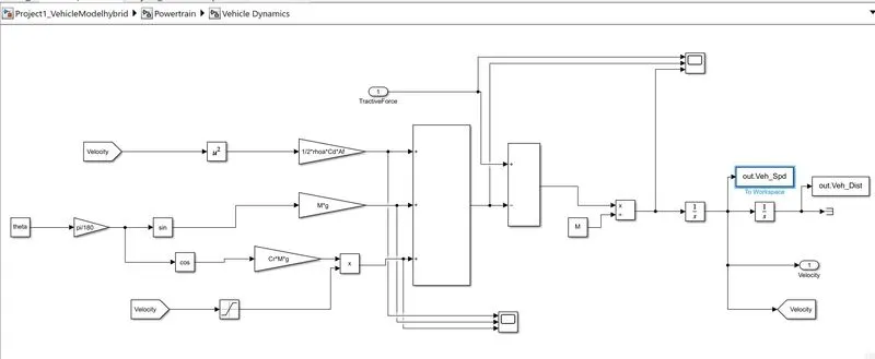
VEHICLE DYNAMICS BLOCK-
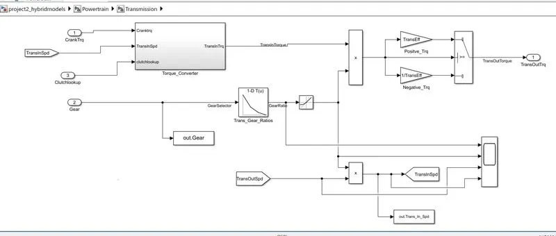
TRANSMISSION BLOCK-
After creating the model,the results can be obtained by running the processing file script.
The processing script is given below-
%% Renaming variables
Time = out.tout;
Acc_Pdl = out.Acc_Pdl; % Accelerator pedal [%]
Brk_Pdl = out.Brk_Pdl; % Brake pedal [%]
Gear = out.Gear; % Transmission gear
Trans_In_Spd = out.Trans_In_Spd*30/pi; % Transmission input speed [rpm]
Trans_Out_Spd = out.Trans_Out_Spd*30/pi;% Transmission output speed [rpm]
Eng_Trq = out.Eng_Trq; % Engine brake torque [Nm]
Eng_Spd = out.Eng_Spd*30/pi; % Engine speed [rpm]
Eng_Fuel_Consump = out.Eng_Fuel_Consumption; % Engine fuel consumption [g]
Eng_fuelrate = out.Eng_Fuel_Rate;
Veh_Dist = out.Veh_Dist/1000; % Distance traveled by vehicle [km]
Veh_Spd = out.Veh_Spd*18/5; % Vehicle speed [kmph]
wheel_spd = out.WheelSpd;
Eng_Fuel_Rate = out.Eng_Fuel_Rate; % Engine fuel rate [%]
EM_Speed = out.emspd*18/5; % Electric Motor Speed
EM_Power = out.Elecpwr; % Electric Motor Power
EM_Torque = out.Emtrq; % Electric Motor Torque
Term_Volt = out.terminal_voltage; % Terminal Voltage of battery
Soc = out.soc; % State Of Charge
Pack_Current = out.packcurrent; %Pack current of battery
%% Data Analysis
Eng_Pwr = Eng_Spd.*pi/30.*Eng_Trq/1000; % Engine brake power [kW]
rho_petrol = 0.7197; % Density of petrol [kg/L]
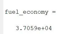
kmpl = Veh_Dist(end)/(Eng_Fuel_Consump(end)/1000/rho_petrol); % Fuel economy [kmpl]
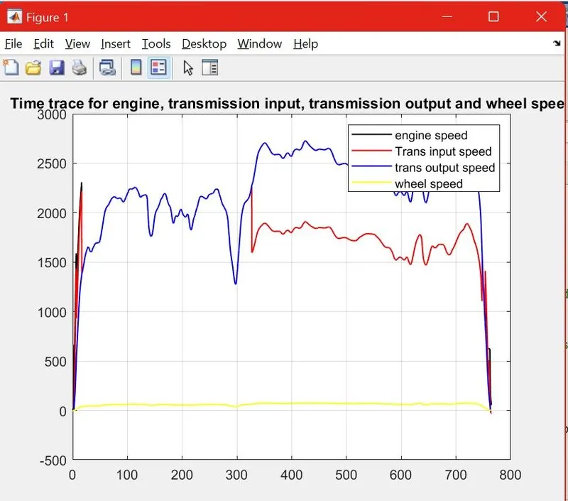
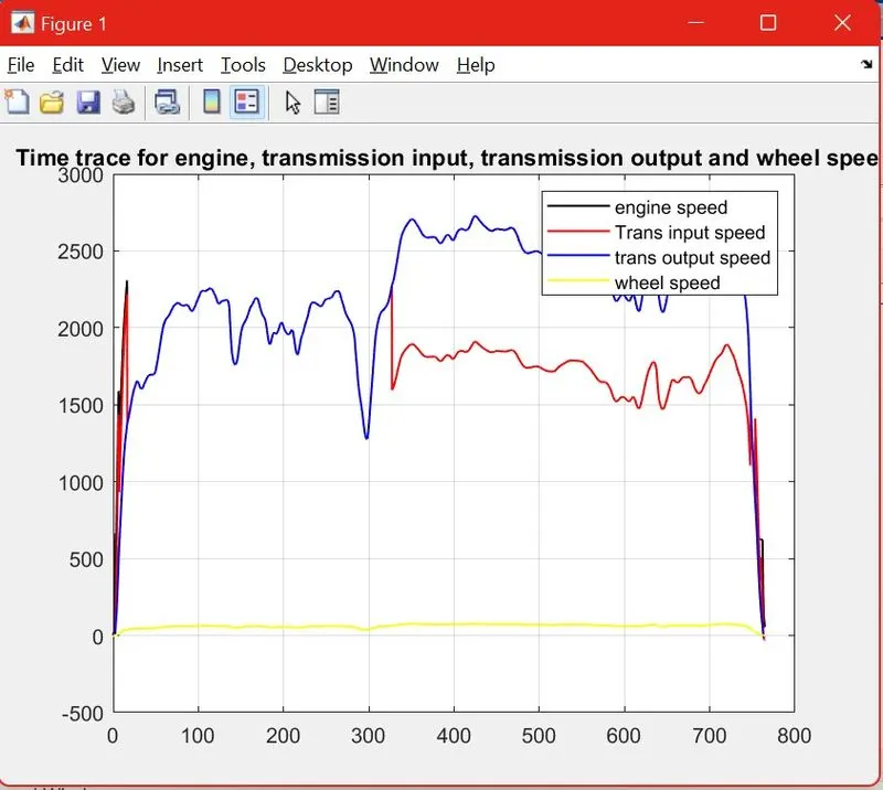
figure(1)
plot(Time,Eng_Spd , 'linewidth', 1, 'Color', 'black')
title('Time trace for engine, transmission input, transmission output and wheel speed')
hold on
plot(Time, Trans_In_Spd, 'linewidth', 1, 'Color', 'red')
plot(Time, Trans_Out_Spd, 'linewidth', 1, 'Color', 'blue')
plot(Time, wheel_spd, 'linewidth', 1, 'Color', 'yellow')
hold off
legend('engine speed','Trans input speed','trans output speed','wheel speed')
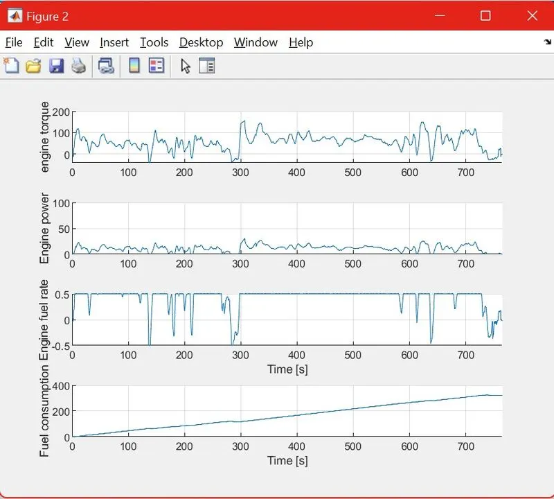
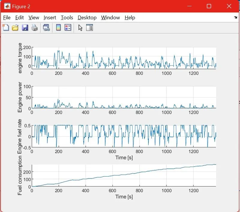
figure(2)
title('Engine torque, engine power, fuel rate and fuel consumption');
subplot(4,1,1)
hold on
grid on
plot(Time, Eng_Trq);
ylabel('engine torque')
xlim([0, Time(end)]);
subplot(4,1,2)
hold on
grid on
plot(Time, Eng_Pwr);
ylabel('Engine power')
xlim([0, Time(end)]);
ylim([0, 100]);
subplot(4,1,3)
hold on
grid on
plot(Time, Eng_fuelrate);
xlim([0, Time(end)]);
xlabel('Time [s]');
ylabel('Engine fuel rate');
subplot(4,1,4)
hold on
grid on
plot(Time, Eng_Fuel_Consump);
xlim([0, Time(end)]);
xlabel('Time [s]');
ylabel('Fuel consumption');
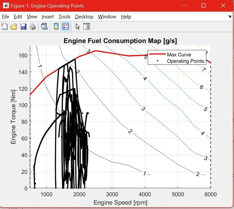
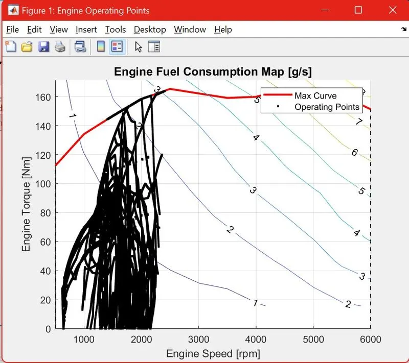
%% Plotting engine operating points on engine fuel map
figure('Name','Engine Operating Points');
hold on
grid on
title('Engine Operating Points','fontsize',12);
p1=plot(Eng_map_spd*30/pi,Eng_max_trq,'linewidth',2,'color','r');
p2=line([Eng_map_spd(end)*30/pi Eng_map_spd(end)*30/pi],[0 Eng_max_trq(end)]);
set(p2,'linewidth',1,'linestyle','--','color','k');
p3=line([Eng_map_spd(1)*30/pi Eng_map_spd(1)*30/pi],[0 Eng_max_trq(1)]);
set(p3,'linewidth',1,'linestyle','--','color','k');
[c,h] = contour(Eng_map_spd'*30/pi,Eng_map_trq,Eng_fuel_map');
clabel(c,h);
xlabel('Engine Speed [rpm]');
ylabel('Engine Torque [Nm]');
title('Engine Fuel Consumption Map [g/s]');
p4 = plot(Eng_Spd,Eng_Trq,'.','color','k');
legend([p1 p4],{'Max Curve','Operating Points'});
axis([Eng_map_spd(1)*30/pi Eng_map_spd(end)*30/pi 0 Eng_map_trq(end)]);
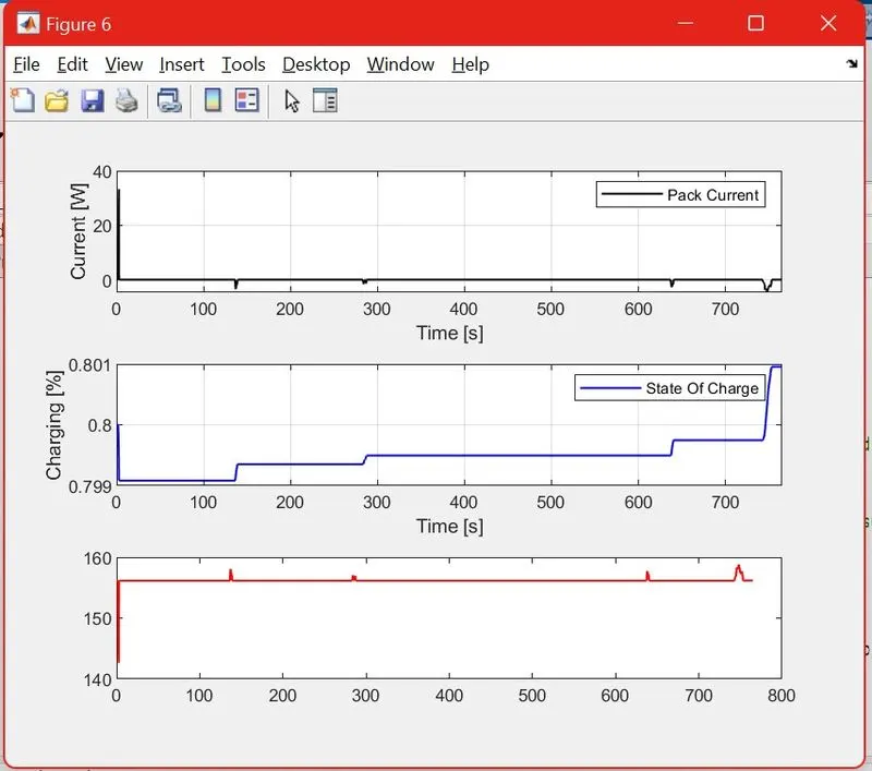
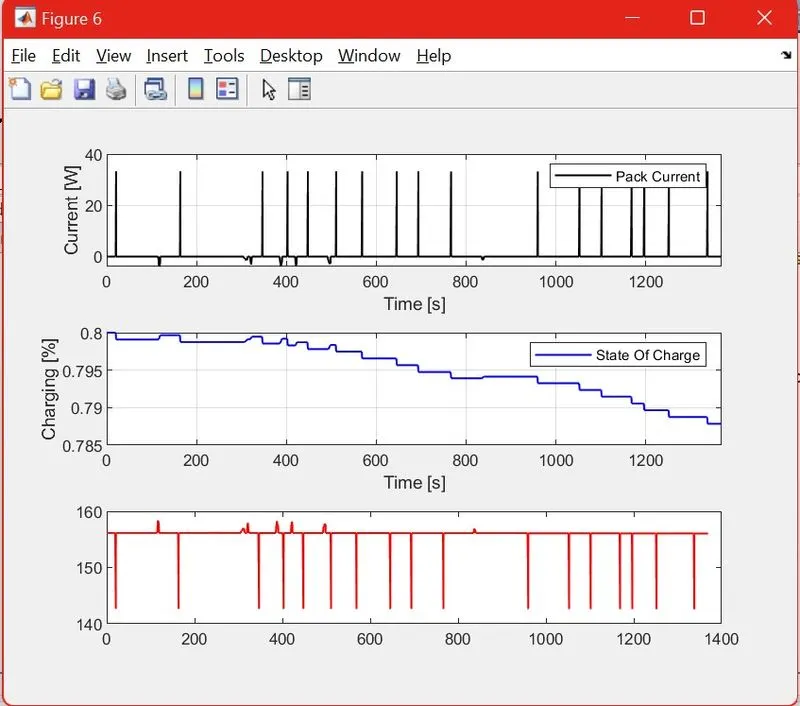
%% State of Charge, Pack Current, And Terminal Voltage with respect to Time
figure(4)
subplot(3,1,1)
plot(Time, Pack_Current,'linewidth',1,'color','black')
xlim([0, Time(end)]);
xlabel('Time [s]')
ylabel('Current [W]')
legend('Pack Current')
grid on
subplot(3,1,2)
plot(Time,Soc,'linewidth',1,'color','blue')
xlim([0, Time(end)]);
xlabel('Time [s]')
ylabel('Charging [%]')
legend('State Of Charge')
grid on
subplot(3,1,3)
plot(Time,Term_Volt,'linewidth',1,'color','red')
xlim([0, Time(end)]);
xlabel('Time [s]')
ylabel('Voltage [V]')
legend('Terminal Voltage')
grid on
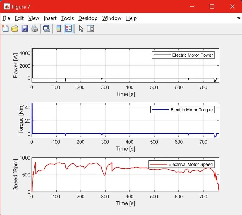
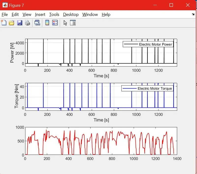
%% Motor Speed, Torque, Motor input power with respect to Time
figure(5)
subplot(3,1,1)
plot(Time,EM_Power,'linewidth',1,'color','black')
xlim([0, Time(end)]);
xlabel('Time [s]')
ylabel('Power [W]')
legend('Electric Motor Power ')
grid on
subplot(3,1,2)
plot(Time,EM_Torque,'linewidth',1,'color','blue')
xlim([0, Time(end)]);
xlabel('Time [s]')
ylabel(' Torque [Nm]')
legend('Electric Motor Torque')
grid on
subplot(3,1,3)
plot(Time,EM_Speed,'linewidth',1,'color','red')
xlim([0, Time(end)]);
xlabel('Time [s]')
ylabel('Speed [Rpm]')
legend('Electrical Motor Speed')
grid on
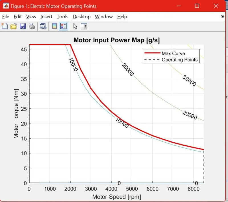
%% Plotting EM Operating Points on motor input power Map
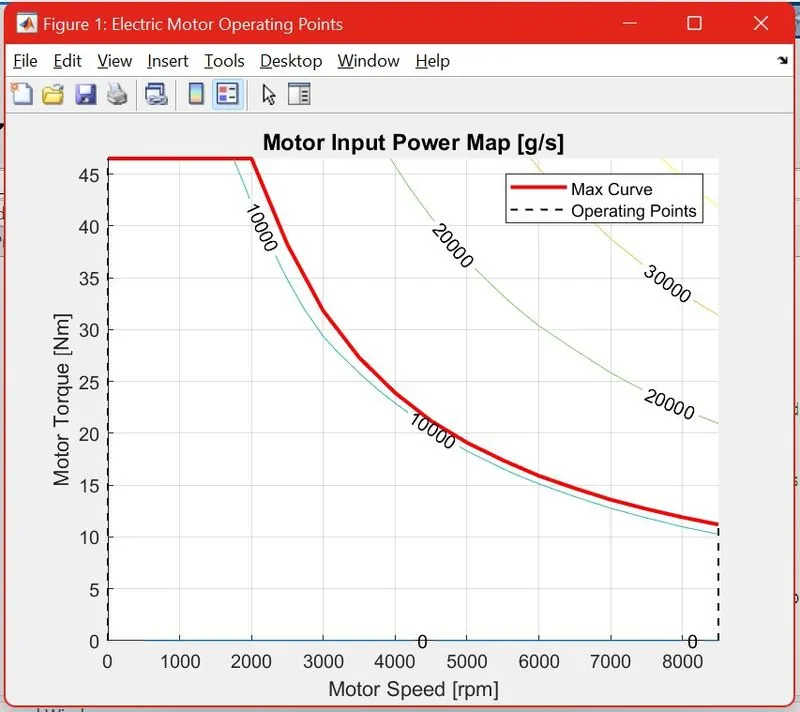
figure('Name','Electric Motor Operating Points');
hold on
grid on
title('Electric Motor Operating Points','fontsize',12);
p1=plot(EM_map_spd*30/pi,EM_max_trq,'linewidth',2,'color','r');
p2=line([EM_map_spd(end)*30/pi EM_map_spd(end)*30/pi],[0 EM_max_trq(end)]);
set(p2,'linewidth',1,'linestyle','--','color','k');
p3=line([EM_map_spd(1)*30/pi EM_map_spd(1)*30/pi],[0 EM_max_trq(1)]);
set(p3,'linewidth',1,'linestyle','--','color','k');
[c,h] = contour(EM_map_spd'*30/pi,EM_map_trq,EM_inpwr_map');
clabel(c,h);
xlabel('Motor Speed [rpm]');
ylabel('Motor Torque [Nm]');
title('Motor Input Power Map [g/s]');
legend([p1 p3],{'Max Curve','Operating Points'});
axis([EM_map_spd(1)*30/pi EM_map_spd(end)*30/pi 0 EM_map_trq(end)]);
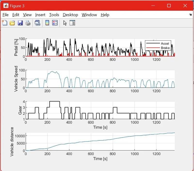
figure(7)
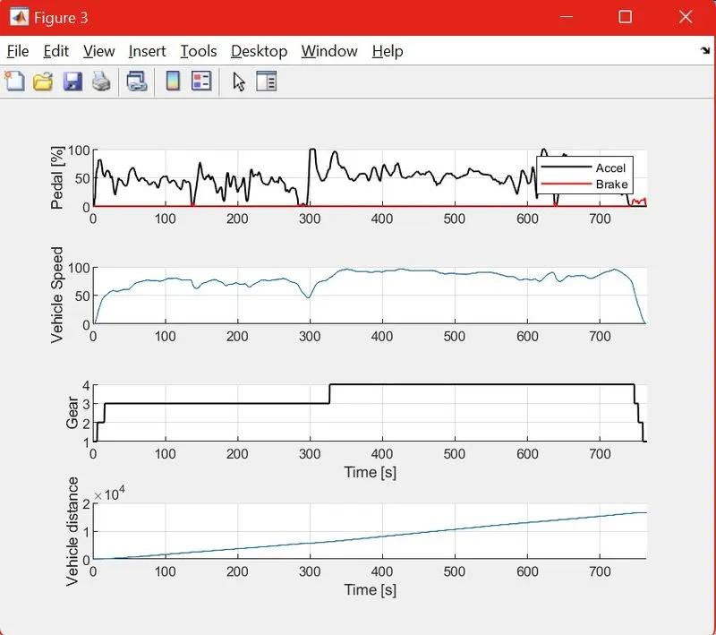
title('Accelerator and brake pedal, gear command, vehicle actual speed, vehicle distance');
subplot(4,1,1)
hold on
grid on
plot(Time, Acc_Pdl, 'linewidth', 1, 'Color', 'black');
plot(Time, Brk_Pdl, 'linewidth', 1, 'Color', 'red');
ylabel('Pedal [%]')
xlim([0, Time(end)]);
legend('Accel','Brake');
subplot(4,1,2)
hold on
grid on
plot(Time, Veh_Spd);
ylabel('Vehicle Speed')
xlim([0, Time(end)]);
ylim([0, 100]);
subplot(4,1,3)
hold on
grid on
plot(Time, Gear, 'linewidth', 1, 'Color', 'black');
xlim([0, Time(end)]);
xlabel('Time [s]');
ylabel('Gear');
subplot(4,1,4)
hold on
grid on
plot(Time, Veh_Dist);
xlim([0, Time(end)]);
xlabel('Time [s]');
ylabel('Vehicle distance');
The results obtained for UDDS and HWFET are given below-
1.UDDS CYCLE
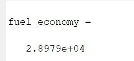
2.HWFET CYCLE