Project 1
The initialization script is run to load up the variables in the workspace.
The script is given below-
%% Vehicle Parameters
M = 1500; % Vehicle weight [kg]
Cr = 0.015; % Rolling resistance coefficient
Rw = 0.35; % Rolling radius [m]
Cd = 0.33; % Drag coefficient
Af = 2; % Frontal area [m2]
rhoa = 1.225; % Air density [kg/m3]
Vwind = 0; % Wind velocity [kmph]
g = 9.81; % Gravitational acceleration [m/s2]
theta = 0; % Slope [deg]
myu_road_tire = 1; % Coefficient of friction between tire - road interface
%% Powertrain Parameters
FDR = 3.73; % Final Drive Ratio / Diff Ratio
DiffEff = 0.99; % Differential efficiency (assumed independent of operating conditions)
NumGear = 4; % Number of gears in transmission
TransGear = [1:NumGear]; % Transmission Gears
TransRatio = [3.06, 1.62, 1, 0.7]; % Corresponding Transmission ratios
TransEff = 0.90; % Transmission efficiency (assumed independent of operating conditions)
TC_SR = [0, .5, .6, .7, .8, .87, .92, .94, .96, .97, 1]; % Torque Converter Speed Ratio (Matlab default) -> TurbSpd/PumpSpd
TC_TR = [2.232, 1.5462, 1.4058, 1.2746, 1.1528, 1.0732, 1.0192, 1, 1, 1, 1]; % Torque Converter Torque Ratio (Matlab default) -> TurbTrq/PumpTrq
TC_Cf = 1e-4 * [.72558, .66322, .63463, .59042, .51331, .4144, .29287, .22444, .12186, .04386, 0]; % Torque Converter Capacity Factor (Matlab default) -> PumpTrq/PumpSpd^2 [Nm/rpm^2]
load Vehicle_Data/Engine_data_1_9L_Saturn_95kW
load Vehicle_Data/Trans_Shift_map
%% Driver Parameters
Kp = 10; % P gain for driver PI model
Ki = 1; % I gain for driver PI model
Drive_Cycle_Select = 2; % Drive cycle selection
% Drive cycle values in m/s
if Drive_Cycle_Select == 1
load DriveCycles/UDDS;
elseif Drive_Cycle_Select == 2
load DriveCycles/HWFET;
elseif Drive_Cycle_Select == 3
load DriveCycles/FTP;
elseif Drive_Cycle_Select == 4
load DriveCycles/US06;
elseif Drive_Cycle_Select == 5
load DriveCycles/NEDC;
elseif Drive_Cycle_Select == 6
load DriveCycles/WLTP;
end
time_end = cyc_time(end);
vel_end = cyc_vel(end);
The simulink model of the conventional vehicle is created ,it references the variables in the workspace.
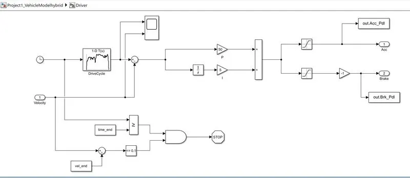
DRIVER BLOCK-
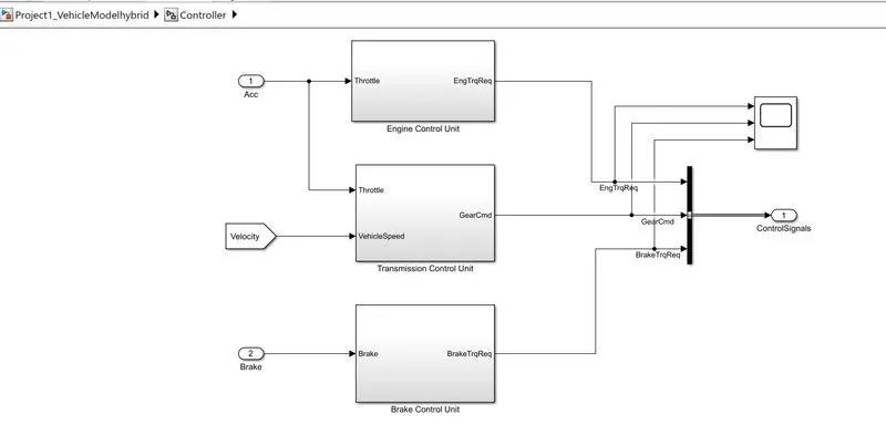
CONTROLLER BLOCK-
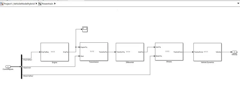
POWERTRAIN BLOCK-
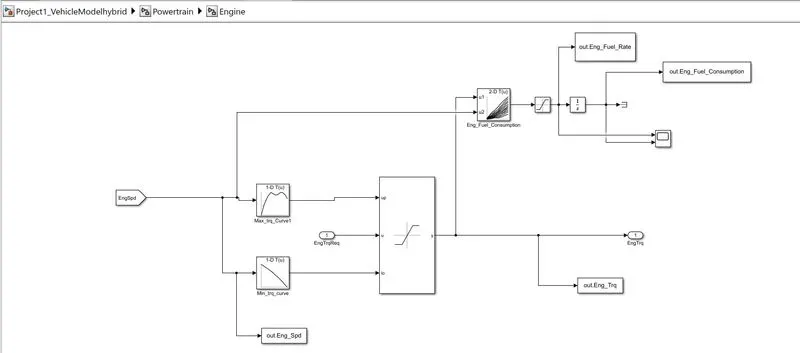
ENGINE BLOCK IN POWERTRAIN-
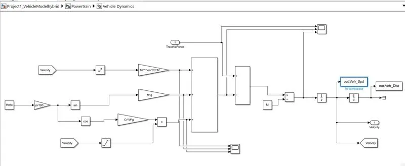
VEHICLE DYNAMICS BLOCK IN POWERTRAIN-
After creating the model,the results can be obtained by running the processing file script.
The processing script is given below-
%% Renaming variables
Time = out.tout;
Acc_Pdl = out.Acc_Pdl; % Accelerator pedal [%]
Brk_Pdl = out.Brk_Pdl; % Brake pedal [%]
Gear_Cmd = out.Gear_Cmd; % Transmission gear
Trans_In_Spd = out.Trans_In_Spd*30/pi; % Transmission input speed [rpm]
Trans_Out_Spd = out.Trans_Out_Spd*30/pi;% Transmission output speed [rpm]
Eng_Trq = out.Eng_Trq; % Engine brake torque [Nm]
Eng_Spd = out.Eng_Spd*30/pi; % Engine speed [rpm]
Eng_Fuel_Consump = out.Eng_Fuel_Consumption; % Engine fuel consumption [g]
Eng_fuelrate = out.Eng_Fuel_Rate;
Veh_Dist = out.Veh_Dist/1000; % Distance traveled by vehicle [km]
Veh_Spd = out.Veh_Spd*18/5; % Vehicle speed [kmph]
wheel_spd = out.WheelSpd;
%% Data Analysis
Eng_Pwr = Eng_Spd.*pi/30.*Eng_Trq/1000; % Engine brake power [kW]
rho_petrol = 0.7197; % Density of petrol [kg/L]
kmpl = Veh_Dist(end)/(Eng_Fuel_Consump(end)/1000/rho_petrol) % Fuel economy [kmpl]
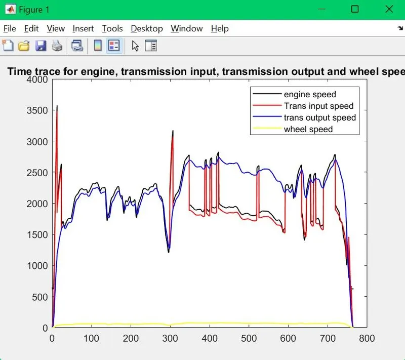
figure(1)
title('Engine speed, transmission input speed, transmission output speed and wheel speed','fontsize',12);
plot(Time,Eng_Spd , 'linewidth', 1, 'Color', 'black')
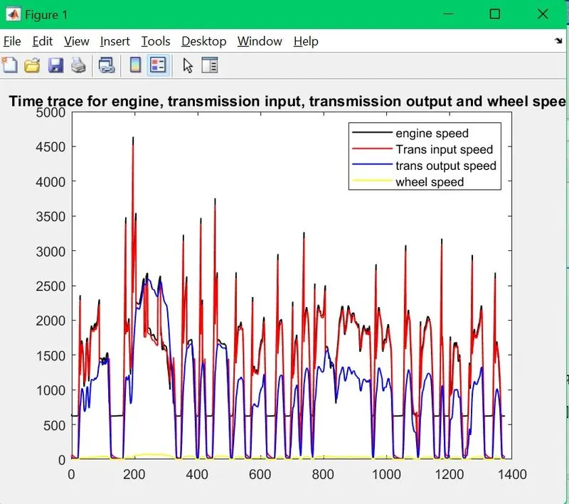
title('Time trace for engine, transmission input, transmission output and wheel speed')
hold on
plot(Time, Trans_In_Spd, 'linewidth', 1, 'Color', 'red')
plot(Time, Trans_Out_Spd, 'linewidth', 1, 'Color', 'blue')
plot(Time, wheel_spd, 'linewidth', 1, 'Color', 'yellow')
hold off
legend('engine speed','Trans input speed','trans output speed','wheel speed')
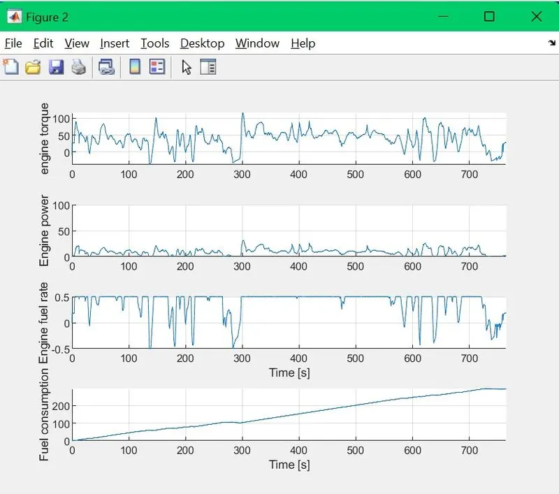
figure(2)
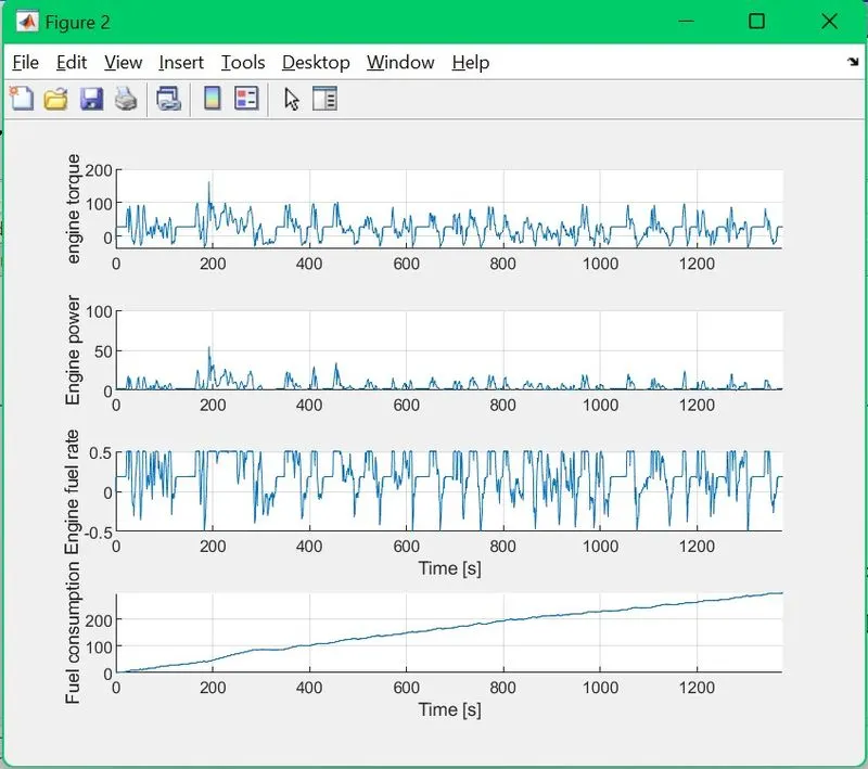
title('Engine torque, engine power, fuel rate and fuel consumption');
subplot(4,1,1)
hold on
grid on
plot(Time, Eng_Trq);
ylabel('engine torque')
xlim([0, Time(end)]);
subplot(4,1,2)
hold on
grid on
plot(Time, Eng_Pwr);
ylabel('Engine power')
xlim([0, Time(end)]);
ylim([0, 100]);
subplot(4,1,3)
hold on
grid on
plot(Time, Eng_fuelrate);
xlim([0, Time(end)]);
xlabel('Time [s]');
ylabel('Engine fuel rate');
subplot(4,1,4)
hold on
grid on
plot(Time, Eng_Fuel_Consump);
xlim([0, Time(end)]);
xlabel('Time [s]');
ylabel('Fuel consumption');
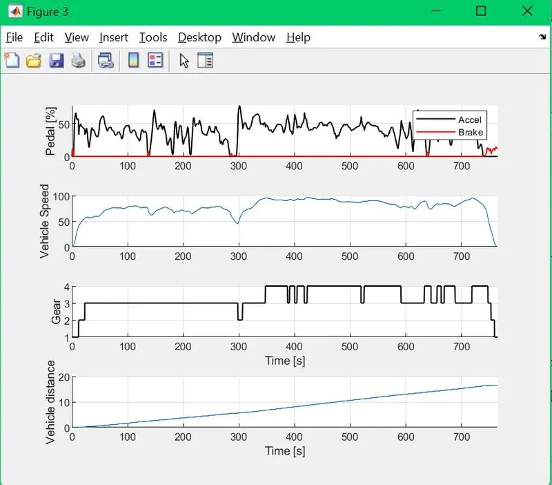
figure(3)
title('Accelerator and brake pedal, gear command, vehicle actual speed, vehicle distance');
subplot(4,1,1)
hold on
grid on
plot(Time, Acc_Pdl, 'linewidth', 1, 'Color', 'black');
plot(Time, Brk_Pdl, 'linewidth', 1, 'Color', 'red');
ylabel('Pedal [%]')
xlim([0, Time(end)]);
legend('Accel','Brake');
subplot(4,1,2)
hold on
grid on
plot(Time, Veh_Spd);
ylabel('Vehicle Speed')
xlim([0, Time(end)]);
ylim([0, 100]);
subplot(4,1,3)
hold on
grid on
plot(Time, Gear_Cmd, 'linewidth', 1, 'Color', 'black');
xlim([0, Time(end)]);
xlabel('Time [s]');
ylabel('Gear');
subplot(4,1,4)
hold on
grid on
plot(Time, Veh_Dist);
xlim([0, Time(end)]);
xlabel('Time [s]');
ylabel('Vehicle distance');
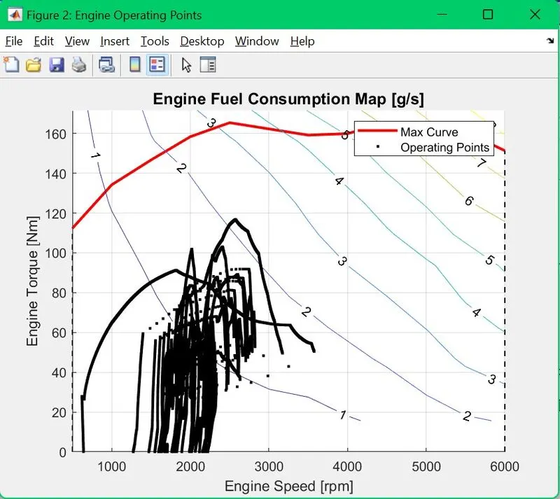
%% Plotting engine operating points on engine fuel map
figure('Name','Engine Operating Points');
hold on
grid on
title('Engine Operating Points','fontsize',12);
p1=plot(Eng_map_spd*30/pi,Eng_max_trq,'linewidth',2,'color','r');
p2=line([Eng_map_spd(end)*30/pi Eng_map_spd(end)*30/pi],[0 Eng_max_trq(end)]);
set(p2,'linewidth',1,'linestyle','--','color','k');
p3=line([Eng_map_spd(1)*30/pi Eng_map_spd(1)*30/pi],[0 Eng_max_trq(1)]);
set(p3,'linewidth',1,'linestyle','--','color','k');
[c,h] = contour(Eng_map_spd'*30/pi,Eng_map_trq,Eng_fuel_map');
clabel(c,h);
xlabel('Engine Speed [rpm]');
ylabel('Engine Torque [Nm]');
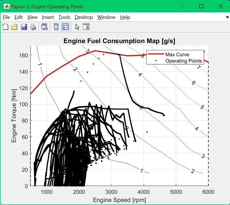
title('Engine Fuel Consumption Map [g/s]');
p4 = plot(Eng_Spd,Eng_Trq,'.','color','k');
legend([p1 p4],{'Max Curve','Operating Points'});
axis([Eng_map_spd(1)*30/pi Eng_map_spd(end)*30/pi 0 Eng_map_trq(end)]);
The results obtained for UDDS and HWFET are given below-
1.UDDS CYCLE
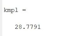
The kmpl for udds cycle is found to be 28.77
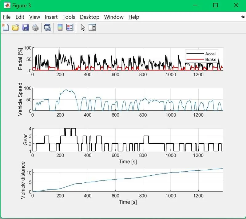
2.HWFET CYCLE
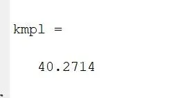
kmpl for hwfet cycle is found to be 40.27