Project 2
DEVELOPMENT OF A FORWARD ENERGY BASED FUEL CONSUMPTION MODEL OF A P1 HYBRID VEHICLE
OBJECTIVE:
The main goal of this project is to understand the functionality of a P1 hybrid and be able to model it.
The objective of this project is to quantify the improvement in fuel economy numbers for the hybrid vehicle (kmpl), compared to the conventional vehicle, on the urban cycle (UDDS) and highway cycle (HWFET). Also, to analyze and understand the vehicle operating points in terms of engine and motor speed, torque, transmission speeds, pedal positions, gear, distance traveled, battery voltage, current, SoC etc.
a. Tabulate the fuel economy numbers (kmpl) for UDDS and HWFET cycle. Compare these numbers with the baseline numbers for conventional vehicle model from Project 1.
b. Plot the time trace for engine, transmission input, transmission output and wheel speed on one plot.
c. Plot engine torque, engine power, fuel rate and fuel consumption using subplots.
d. Plot accelerator and brake pedal, gear command, vehicle desired and actual speed, vehicle distance using subplots.
e. Plot the engine operating points on the engine fuel map.
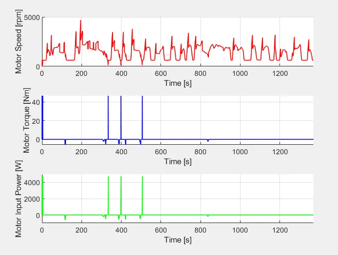
f. Plot motor speed, torque, motor input power using subplots.
g. Plot pack voltage, current and SoC using subplots.
h. Plot the motor operating points on the motor input power map, with the motor max motoring and generating torque curves.
i. Write down appropriate brief comments on each of these plots, describing the vehicle behavior throughout the drive cycle.
j. Generate the plots for both drive cycles
INTRODUCTION:
Mild hybrids—also called micro hybrids—use a battery and electric motor to help power the vehicle and can allow the engine to shut off when the vehicle stops (such as at traffic lights or in stop-and-go traffic), further improving fuel economy. Mild hybrid systems cannot power the vehicle using electricity alone.
Automotive OEMs and automotive Tier 1 system suppliers are currently analyzing and evaluating several major powertrain architectures for MHEVs. The electric machine can be positioned, relative to the other powertrain components, in five major points:
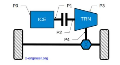
The brief description of the electric machine connection points is done in the table below.
| P0 | The electric machine is connected with the internal combustion engine through a belt, on the front end accessory drive (FEAD) |
| P1 | The electric machine is connected directly with the crankshaft of the internal combustion engine |
| P2 | The electric machine is side-attached (through a belt) or integrated between the internal combustion engine and the transmission; the electric machine is decoupled from the ICE and it has the same speed of the ICE (or multiple of it) |
| P3 | The electric machine is connected through a gear mesh with the transmission; the electric machine is decoupled from the ICE and it’s speed is a multiple of the wheel speed |
| P4 | The electric machine is connected through a gear mesh on the rear axle of the vehicle; the electric machine is decoupled form the ICE and it’s located in the rear axle drive or in the wheels hub |
Notice that P0 and P1 architectures do not allow the mechanical disconnection of the electric machine from the engine. On the other side P2, P3 or P4 configurations disconnects the electric machine from the engine through a clutch.
P1 Hybrid:
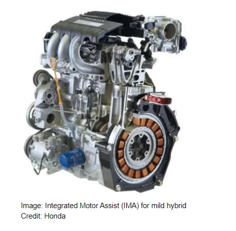
The P1 architecture, with the electric machine connected directly to the crankshaft, is the solution adopted by Honda on their first generation Integrated Motor Assist (IMA) technology. The electric motor functions as a generator, during vehicle deceleration, as an engine starter, and as a motor (to assist the engine) during vehicle accelerations.
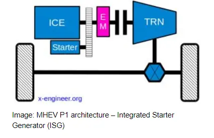
One of the biggest advantage of this solution is that the electric motor can provide higher torque than the BiSG, since there is no belt limitation (due to slip). However, since there is no speed / torque ratio between the electric machine and crankshaft, the torque requirements on the electric motor can be quite demanding.
Two examples of P1 MHEV architectures are:
- Honda Insight Hybrid 2009 (with Integrated Motor Assist technology)
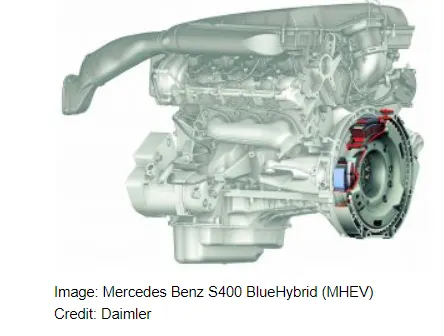
- Mercedes Benz S400 Bluehybrid 2010
Overall characteristics:
Torque Boosting Capability: High (if electric machine is capable)
Electrical Energy Recuperation: Medium (due to engine losses)
Driveability Improvements: Medium (depending on the torque capability of the electric machine)
Electrical Creep / Drive: Possible (depending on the torque capability of the e-machine)
Packaging: Difficult components integration (powertrain specially designed for this architecture)
System Efficiency: High (no gear mesh or belt losses)
FORWARD BASED MODEL FOR A HYBRID VEHICLE:
Forward model:
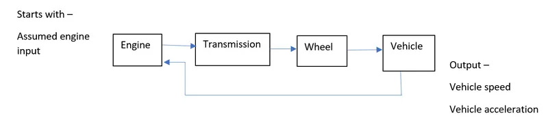
- Forward models are a dynamic simulation, dynamic models are used for detailed simulations.
- Force/torque/power is the input and the vehicle state variables velocity and acceleration are outputs.
- Models and simulation are more realistic due to physical causality, hence appropriate for control development.
- There is a feedback loop to meet the desired vehicle state.
- Slower simulation due to the dynamics.
- Approach mainly used to simulate a vehicle on a driving cycle, to analyze the dynamic behaviour of the system, helps significantly in control development.
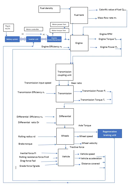
FORWARD MODEL OF HYBRID VEHICLE:
METHODOLOGY:
In this project, we are using forward based model of P1 hybrid vehicle for finding fuel consumption and fuel economy numbers of the vehicle for different drive cycles.
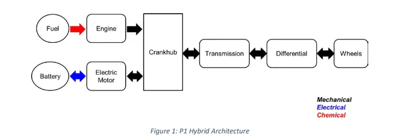
Here,Honda Insight motor and battery are considered for this project. Data is taken from ADVISOR data base developed by NREL, USA.
Motor Used : 10 kW PMSM
Battery used: 6Ah 154V NiMH Battery pack
System Level Configurations:
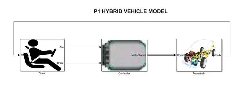
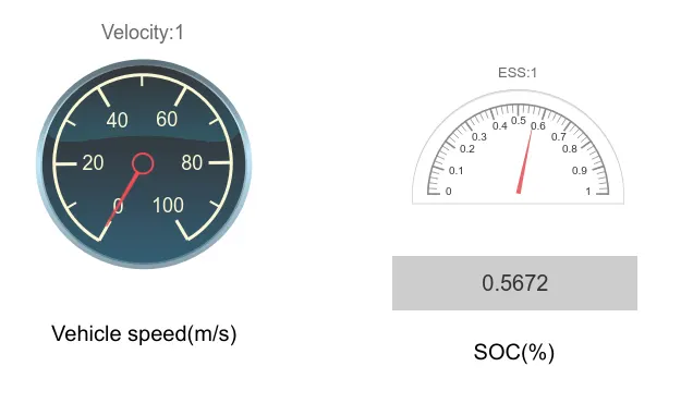
The simulink model mainly consist of three main blocks
Driver Block
Controller Block
Powertrain Block
SIMULINK MODEL:
MODEL INITIALIZATION:
Initialization is done by loading the MATLAB script “Project2_InitFile.m” , this will load all the variables required for running the Simulink model and for post-processing. The drive cycle selection is also done here. Before running the Simulink vehicle model, we need to run this initialization script.
MATLAB code for Initialization:
%%%%%%%%%%%%%%%%%%%%%%%%%%%%%%%%%%%%%%%%%%%%%%%%%%%%%%%%%%%%%%%%%%%%%
%% Skill-Lync -> Hybrid Drives Development
% Project 2 - Forward based model of P1 hybrid vehicle
% By - Riyaz B

% Description:

%% Initialization File
% Initialization file for loading the variables for the Conventional vehicle simulation model

%% Vehicle Parameters
M = 1500;       % Vehicle weight [kg]
Cr = 0.015;     % Rolling resistance coefficient
Rw = 0.35;      % Rolling radius [m]
Cd = 0.33;      % Drag coefficient
Af = 2;         % Frontal area [m2]
rhoa = 1.225;   % Air density [kg/m3]
Vwind = 0;      % Wind velocity [kmph]
g = 9.81;       % Gravitational acceleration [m/s2]
theta = 0;      % Slope [deg]
myu_road_tire = 1; % Coefficient of friction between tire - road interface

%% Powertrain Parameters
FDR = 3.73;                         % Final Drive Ratio / Diff Ratio
DiffEff = 0.99;                     % Differential efficiency (assumed independent of operating conditions)

NumGear = 4;                        % Number of gears in transmission
TransGear = [1:NumGear];            % Transmission Gears
TransRatio = [3.06, 1.62, 1, 0.7];  % Corresponding Transmission ratios
TransEff = 0.90;                    % Transmission efficiency (assumed independent of operating conditions)

TC_SR = [0, .5, .6, .7, .8, .87, .92, .94, .96, .97, 1];   % Torque Converter Speed Ratio (Matlab default) -> TurbSpd/PumpSpd
TC_TR = [2.232, 1.5462, 1.4058, 1.2746, 1.1528, 1.0732, 1.0192, 1, 1, 1, 1];   % Torque Converter Torque Ratio (Matlab default) -> TurbTrq/PumpTrq
TC_Cf = 1e-4 * [.72558, .66322, .63463, .59042, .51331, .4144, .29287, .22444, .12186, .04386, 0]; % Torque Converter Capacity Factor (Matlab default) -> PumpTrq/PumpSpd^2 [Nm/rpm^2]

load Vehicle_Data/Engine_data_1_9L_Saturn_95kW
load Vehicle_Data/Trans_Shift_map
load Vehicle_Data/EM_Honda_Insight_10kW
load Vehicle_Data/ESS_NiMH6


ESS_init_soc = 0.8;
ESS_soc_max = 0.9;
ESS_soc_min = 0.6;


%% Driver Parameters
Kp = 10;                    % P gain for driver PI model
Ki = 1;                     % I gain for driver PI model
Drive_Cycle_Select = 1;     % Drive cycle selection

% Drive cycle values in m/s

if Drive_Cycle_Select == 1
    load DriveCycles/UDDS;

elseif Drive_Cycle_Select == 2
    load DriveCycles/HWFET;

elseif Drive_Cycle_Select == 3
    load DriveCycles/FTP;

elseif Drive_Cycle_Select == 4
    load DriveCycles/US06;

elseif Drive_Cycle_Select == 5
    load DriveCycles/NEDC;

elseif Drive_Cycle_Select == 6
    load DriveCycles/WLTP;

end

time_end = cyc_time(end);
vel_end = cyc_vel(end);
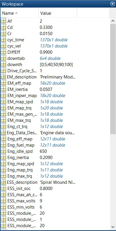
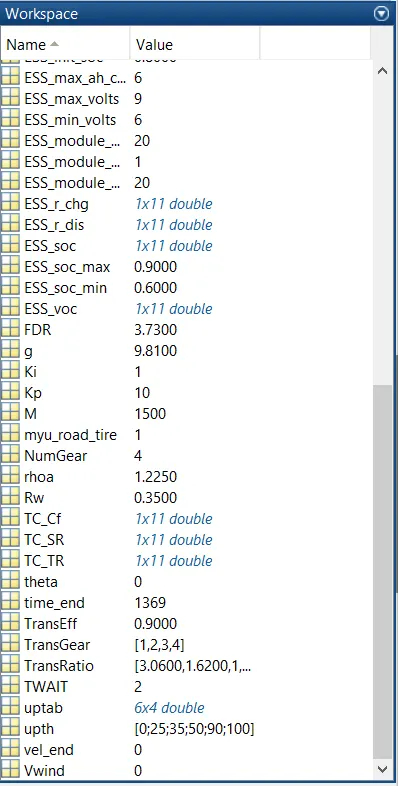
After running this we get the below results in workspace
SIMULINK MODELS:
DRIVER MODEL:
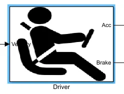
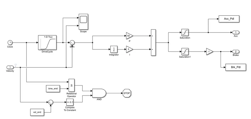
Driver model consist of drive cycle 2d lookup table which have the selected drive cycle values and this model uses the PI controller that generates accelerator and brake pedal outputs to match the desired vehicle speed
These acceleration and brake pedal outputs are given to the controllers for controlling the vehicle.
CONTROLLER MODEL:
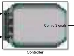
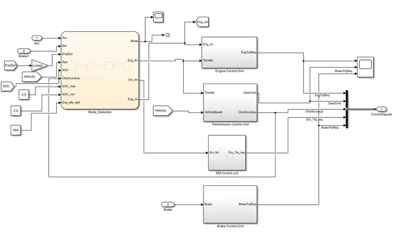
The ‘Controller’ block is the brains of the vehicle, representing the electronic controls units. Based on the driver inputs, it generates desired engine torque, desired transmission gear and desired brake torque, Electric machine torque. These inputs are fed to the ‘Powertrain’ block which represents the drivetrain of the vehicle.
It also consists of supervisory controller which selects the mode of operation.
SUPERVISORY CONTROLLER:
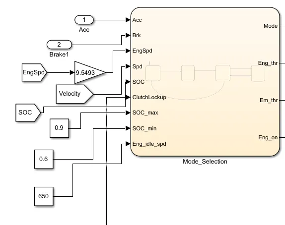
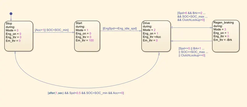
Supervisory controller control the vehicle by using 4 modes stop,start,drive and regenerative braking.
The inputs to the supervisory controller is acceleration,brake signals,engine speed, velocity of the vehicle, state of charge of the battery, max and min soc's,idle speed rpm and clutchlockup signal. based on these inputs it will control the vehicle and made to run vehicle in desired modes.
The output of the block is engine throttle positions, electric machine throttle positions,engine on and off conditions. these outputs are fed to the other controller units.
The stateflow blocks consists of logics if Acc is greater than 1 and soc
ENGINE CONTROL UNIT:
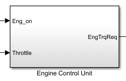
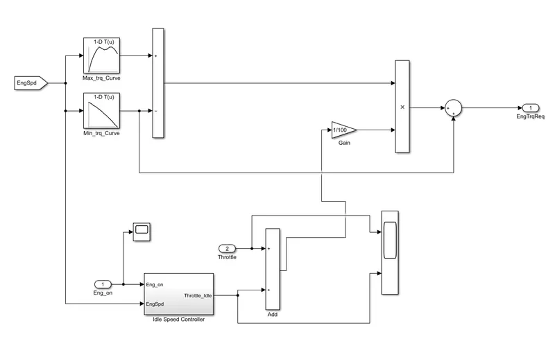
This block consist of 2 1-d lookup tables one with eng max torque and eng map speed and other with eng ct torque and eng map speed which is subtracted and the output is multiplied with idle throttle speed to get the required engine torque requirement,Idle speed controller subsystem consist of PI controller which gives the output of idle throttle speed.
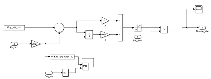
IDLE SPEED CONTROLLER:
The idle speed controller block consist of PI controller which controls the idle speed, In this model the engine idle speed is 650 rpm, engine on mode is given as input to control the engine on and off using the logics and give the throttle idle output. Throttle is multiplied with the torqe requirement to give the desired engine torque requirement.
TRANSMISSION CONTROL UNIT:
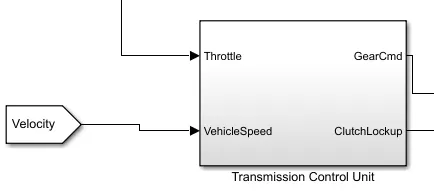
This input is vehicle speed to this stateflow and output is the gear command,the stateflow control block have the shift logic conditions which changes the gears according to the required vehicle speeds and throttle commands with respect to time.
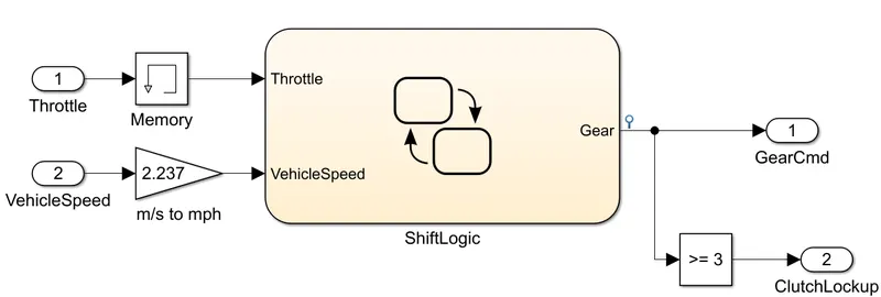
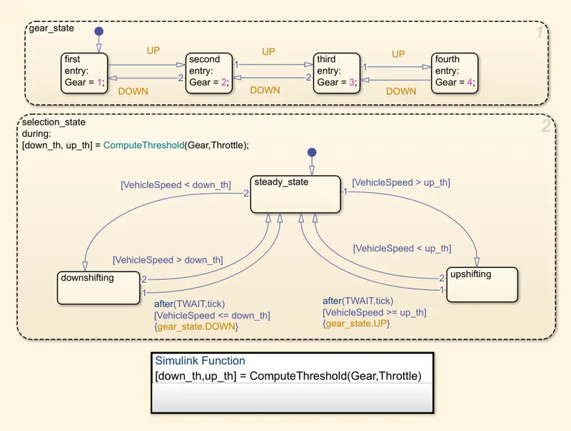
4 speed gear is used here,the stateflow will change the gear by the down throttle and up throttle commands.
below is the stateflow logic for the tranmission unit.
ELECTRIC MACHINE CONTROL UNIT:
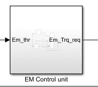
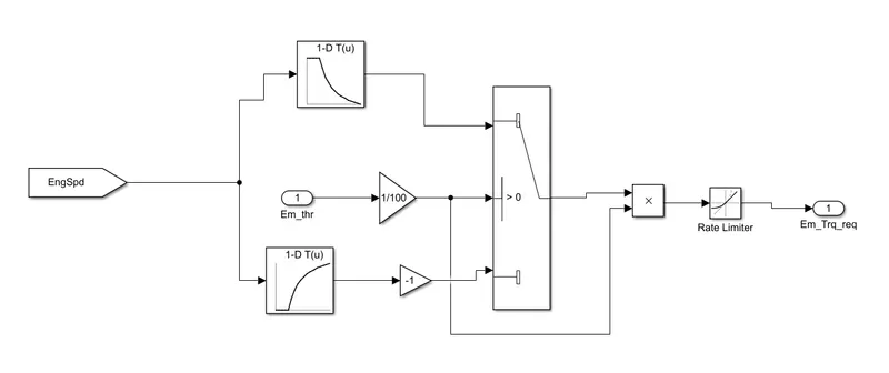
Electric machine control unit uses the engine speed as reference and it uses 2 lookup tables one with motor max torque and anothr with motor regeneration torque and we get the motor torque requirement as output.rate limiter is used here to limit the rate of torque requirement.
BRAKE CONTROL UNIT:
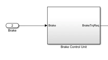
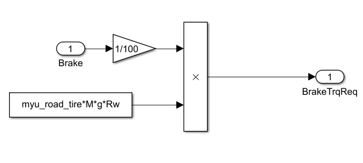
This block gives the brake torque by computing the brake torque formula
myu_road_tire*M*g*Rw
this control block gives the brake torqe requirement as output.
POWERTRAIN BLOCK:
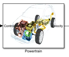
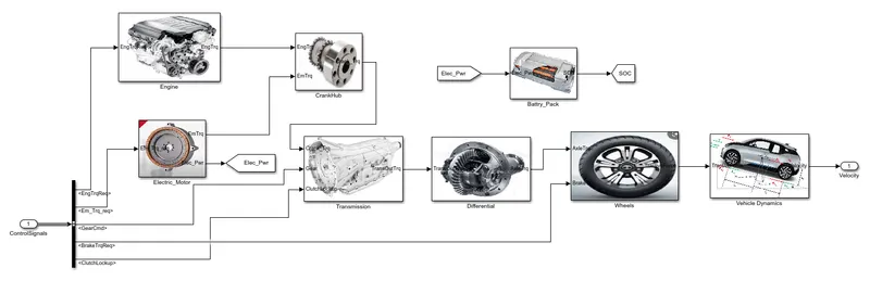
‘Powertrain’ block which represents the drivetrain of the vehicle. It consists of an ‘Engine’ 'Electric Motor' and crank hub connected to the ‘Automatic Transmission’ through a ‘Torque Converter’. The output of the transmission is connected to the ’Differential’, which powers the ‘Wheels’, that provides the tractive force for vehicle acceleration. The longitudinal dynamics of the vehicle along with the road load is represented in the ‘Vehicle Dynamics’ block.
ENGINE BLOCK:
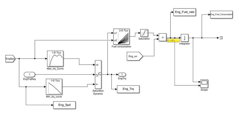
In this Engine model we used map based model to find out the engine fuel consumption and engine fuel rate,engine speed and saturated torque from the map model is taken to the 2d lookup table which then saturated and integrated to get the engine fuel consumption and engine fuel rate. By integrating the engine fuel rate we get the engine fuel consumption.
Eng on and off mode is added to off the engine while vehicle in idle and then start if the vehicle is on drive mode.
ELECTRIC MOTOR BLOCK:
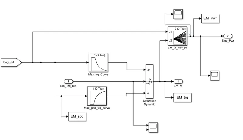
Map based model is created for the electric motor to get the electric power requirement 2 lookup table is used here with electric motor torque and speed and other one with electric generative torque and speed, electric power is calculated sing the 2D lookup table which have the electric machine input power based on the motor speed and torque. To workspace block is used to get he otput motor power,motor speed,motor torque to the workspace.
CRANK HUB BLOCK:
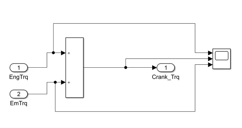
Crank hub block where the engine and motor torque is added and the crank torque is given as output. the crank torque is given to the transmission unit as input.
TRANSMISSION BLOCK:
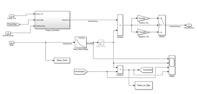
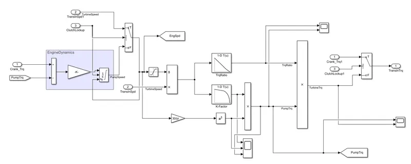
Crank torque and gear command is input to the transmission block which is computed to get the desired transmission output toque as output,Torque converter subsystem consist of engine dynamics block,pump and turbine,in which the pump torque and turbine torque,k factor is used to find out the desired transmission input torque.
Transmission input torque and transmission gear ratio is multiplied to get the transmission efficiency after that positive torque and negative torque values are separated using switch block to get the desired transmission output torque.
TORQUE CONVERTER BLOCK:
A torque converter is a type of fluid coupling which is used to transfer rotating power from the engine of a vehicle to the transmission. It takes place of a mechanical clutch in an automatic transmission. The main function of it is to allow the load to be isolated from the main power source. It sits in between the engine and transmission. It has the same function as the clutch in manual transmission. As the clutch separates the engine from the load when it stops, in the same way, it also isolates the engine from the load and keeps engine running when a vehicle stops.
Cars with automatic transmissions don’t have clutches, so they need a way to let the engine keep running while the wheels and gears in the transmission come to a stop. Manual transmission cars use a clutch that disconnects the engine from the transmission. Automatic transmissions use a torque converter.
Here the torque converter block is model using the torque ratio and K-factor. If the clutch lockup is on then the turbine speed is equal to the pump speed.
Here we get the required transmission input torque as the output from the torque converter block.
The transmission block gives the transmission output torque requirement as the output which is then given to the differential block.
DIFFERENTIAL BLOCK:
In this model,transmission output torque is taken as input and fed to the differential,differential efficiency which gives the positive and negative torque from where we get the axle torque.
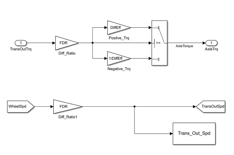
The final drive ratio gives the transmission output speed with reference with the wheel speed.
WHEEL BLOCK:
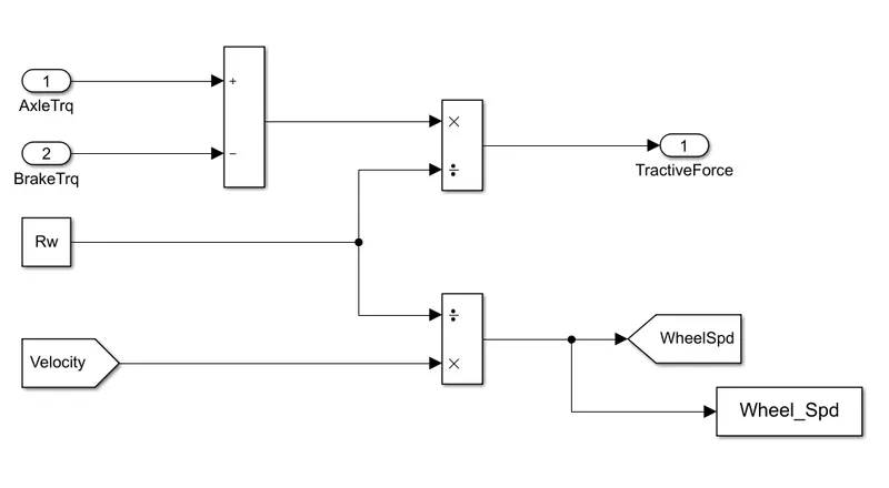
In this model axle torque from differential and brake torque from brake control unit which is subtracted and multiplied with wheel rolling radius and velocity to get the tractive force to drive the wheels and rolling radius and velocity gives the wheel speed.to workspace block is used get the wheel speed to workspace for post processing.
Tractive Force Calculation for a Vehicle : Applied tractive force based on engine torque can be calculated as
TE = (Et x η x Ng x Na ) / R…………………………eq.1
Where,
TE – tractive force in N
Et – Engine torque in Nm
η – Overall efficiency of power train
Ng – Transmission ratio
Na – Driving axle ratio
R – Tire rolling radius
v = ω × R . We can rewrite this expression to obtain the equation of angular velocity.
VEHICLE DYNAMICS BLOCK:
Vehicle dynamics block simply compute the vehicle dynamic equations to get the desired vehicle velocity,vehicle speed and vehicle distance.
Road load formulas computed are given below
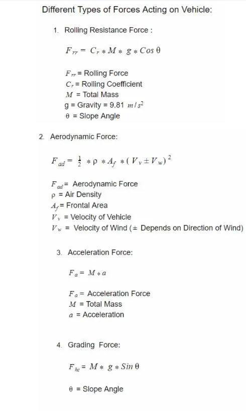
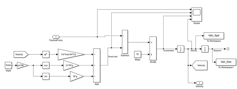
This block will give the out vehicle speed and distance travelled by the vehicle.
BATTERY PACK MODEL:
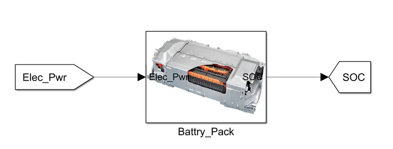
Electric power is the input to the battey pack and state of charge is the output of the battery pack.
SOC and terminal voltage of the battery is estimated by the equivalent circuit model of the battery.
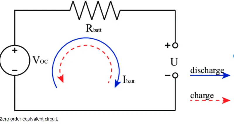
Here,Honda insight 6Ah and 154V NiMH batttery model is used, all the battery parameters such as pack current,soc amx and min,capacity are loaded to the workspace by running the data.
load Vehicle_Data/ESS_NiMH6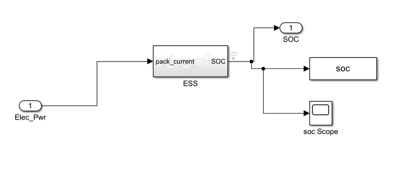
Equivalent circuit model of battery pack:
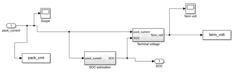
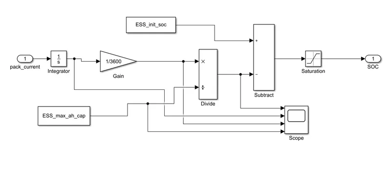
SOC estimation:
SOC is estimated by integrating the current and divide by the capacity and subtract with the initial soc to get the desired soc level of battery pack.
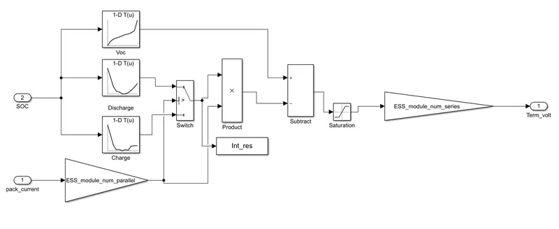
Terminal voltage estimation:
The battery voltage output equation, from the Kirchhoff law, is given by:
Vbatt = Voc − Ibatt · R(internal resistance)
modules in series and parallel are calculated to get the desired output capacity and voltages of the battery pack.
Pre-processing:
Below script is the pre processing file of the model, after running this file it will plot the desired result plots.
this script file file have the scripts to get the output values from simulink file to the workspace and process it and give the desired plots using the plot commands and contour commands.
All the results are plotted in subplots using the subplot commands.
%%%%%%%%%%%%%%%%%%%%%%%%%%%%%%%%%%%%%%%%%%%%%%%%%%%%%%%%%%%%%%%%%%%%%
%% Skill-Lync -> Hybrid Drives Development
% Project 2 - Forward based model of P1 Hybrid
% By - Riyaz B

% Description:
% The following file is to used with the Initialization file and Simulink
% results for post-processing of the data.
% The file is incomplete, has some examples of how the data is imported
% into a readable format, data analysis and plotting examples.
% Based on the project task, use commands in a similar format as given
% below, to analyse the data and generate required plots.
% You can change variable names if desired

%% Post-Processing File
%  File for post-processing the P1 hybrid vehicle simulation model data

%% Renaming variables
Time = out.tout;
Acc_Pdl = out.Acc_Pdl;          % Accelerator pedal [%]
Brk_Pdl = out.Brk_Pdl;          % Brake pedal [%]
Gear_Cmd = out.Gear_Cmd;        % Transmission gear
Trans_In_Spd = out.Trans_In_Spd*30/pi;  % Transmission input speed [rpm]
Trans_Out_Spd = out.Trans_Out_Spd*30/pi;% Transmission output speed [rpm]
Eng_Trq = out.Eng_Trq;          % Engine brake torque [Nm]
Eng_Spd = out.Eng_Spd*30/pi;    % Engine speed [rpm]
Eng_Fuel_Consump = out.Eng_Fuel_Consumption;    % Engine fuel consumption [g]
Veh_Dist = out.Veh_Dist/1000;   % Distance traveled by vehicle [km]
Veh_Spd = out.Veh_Spd*18/5;     % Vehicle speed [kmph]
Wheel_speed = out.Wheel_Spd;
Eng_Fuel_rate = out.Eng_Fuel_rate;
EM_Spd = out.EM_spd*30/pi;
EM_Trq = out.EM_trq;
EM_Power = out.EM_Pwr;
Term_volt = out.term_volt;
SOC = out.soc;
Pack_current = out.pack_crnt;
%% Data Analysis
Eng_Pwr = (Eng_Spd.*pi/30).*(Eng_Trq./1000);   % Engine brake power [kW]
rho_petrol = 0.7197;                    % Density of petrol [kg/L]
kmpl = Veh_Dist(end)/(Eng_Fuel_Consump(end)/1000/rho_petrol);    % Fuel economy [kmpl]

% Display Fuel Economy of the Cycle
fprintf('n fuel economy of drive cycle = %2.2f kmpl ',kmpl)

%% Plotting vehicle characteristics time trace
figure(1)
subplot(3,1,1)
hold on
grid on
plot(Time,Trans_In_Spd, 'linewidth', 1, 'Color', 'black');
ylabel('Speed [rpm]')
xlim([0, Time(end)]);
ylim([0, 6000]);
legend('Trans Input');

subplot(3,1,2)
hold on
grid on
plot(Time, Trans_Out_Spd, 'linewidth', 1, 'Color', 'red');
ylabel('Speed [rpm]')
xlim([0, Time(end)]);
ylim([0, 6000]);
legend('Trans Output');

subplot(3,1,3)
hold on
grid on
plot(Time,Wheel_speed, 'linewidth', 1, 'Color', 'black');
xlim([0, Time(end)]);
xlabel('Time [s]');
ylabel('Wheel speed(m/s)');
legend('wheel speed');


%% plotting engine torque, engine power, fuel rate and fuel consumption using subplots
figure(2)
subplot(4,1,1)
hold on
grid on
plot(Time,Eng_Trq,'linewidth',1,'color','r');
xlim([0, Time(end)]);
xlabel('Time [s]');
ylabel('Engine Torque');

subplot(4,1,2)
hold on
grid on
plot(Time,Eng_Pwr,'linewidth',1,'color','b');
xlim([0, Time(end)]);
xlabel('Time [s]');
ylabel('Engine Power');

subplot(4,1,3)
hold on
grid on
plot(Time,Eng_Fuel_Consump,'linewidth',1,'color','g');
xlim([0, Time(end)]);
xlabel('Time [s]');
ylabel('Engine Fuel consumption');

subplot(4,1,4)
hold on
grid on
plot(Time,Eng_Fuel_rate,'linewidth',1,'color','m');
xlim([0, Time(end)]);
xlabel('Time [s]');
ylabel('Engine Fuel rate');

%% Plot accelerator and brake pedal, gear command, vehicle desired and actual speed,
%% vehicle distance using subplots.
figure(3)
subplot(3,1,1)
hold on
grid on
plot(Time, Acc_Pdl, 'linewidth', 1, 'Color', 'black');
xlabel('Time [s]');
ylabel('Pedal [%]')
xlim([0, Time(end)]);
legend('Accel');

subplot(3,1,2)
hold on
grid on
plot(Time, Brk_Pdl, 'linewidth', 1, 'Color', 'red');
xlabel('Time [s]');
ylabel('Pedal [%]')
xlim([0, Time(end)]);
legend('Brake');

subplot(3,1,3)
hold on
grid on
plot(Time, Gear_Cmd, 'linewidth', 1, 'Color', 'black');
xlim([0, Time(end)]);
xlabel('Time [s]');
ylabel('Gear');
legend('gear cmd');

%vehicle actual and desired speeds and vehicle distance
figure(4)
subplot(3,1,1)
hold on
grid on
plot(Time,Veh_Spd,'linewidth',1,'color','green');
xlim([0, Time(end)]);
xlabel('Time [s]');
ylabel('Vehicle Actual Speed');


subplot(3,1,2)
hold on
grid on
plot(cyc_vel,'linewidth',1,'color','green');
xlim([0, Time(end)]);
xlabel('Time [s]');
ylabel('Vehicle Desired Speed');

subplot(3,1,3)
hold on
grid on
plot(Time,Veh_Dist,'linewidth',1,'color','green');
xlim([0, Time(end)]);
xlabel('Time [s]');
ylabel('Vehicle Distance');

%% Plotting engine operating points on engine fuel map
figure('Name','Engine Operating Points');
hold on
grid on
title('Engine Operating Points','fontsize',12);
p1=plot(Eng_map_spd*30/pi,Eng_max_trq,'linewidth',2,'color','r');
p2=line([Eng_map_spd(end)*30/pi Eng_map_spd(end)*30/pi],[0 Eng_max_trq(end)]);
set(p2,'linewidth',1,'linestyle','--','color','b');
p3=line([Eng_map_spd(1)*30/pi Eng_map_spd(1)*30/pi],[0 Eng_max_trq(1)]);
set(p3,'linewidth',1,'linestyle','--','color','b');
[c,h] = contour(Eng_map_spd'*30/pi,Eng_map_trq,Eng_fuel_map');
clabel(c,h);
xlabel('Engine Speed [rpm]');
ylabel('Engine Torque [Nm]');
title('Engine Fuel Consumption Map [g/s]');
legend([p1 p3],{'Max Curve','Operating Points'});
axis([Eng_map_spd(1)*30/pi Eng_map_spd(end)*30/pi 0 Eng_map_trq(end)]);

% Plot motor speed, torque, motor input power using subplots.
figure(6)
subplot(3,1,1)
hold on
grid on
plot(Time,EM_Spd,'linewidth',1,'color','r');
xlim([0, Time(end)]);
xlabel('Time [s]');
ylabel('Motor Speed [rpm]');

subplot(3,1,2)
hold on
grid on
plot(Time,EM_Trq,'linewidth',1,'color','b');
xlim([0, Time(end)]);
xlabel('Time [s]');
ylabel('Motor Torque [Nm]');

subplot(3,1,3)
hold on
grid on
plot(Time,EM_Power,'linewidth',1,'color','g');
xlim([0,Time(end)]);
ylim([-1000,5000]);
xlabel('Time [s]');
ylabel('Motor Input Power [W]');

% Plot pack voltage, current and SoC using subplots.
figure(7)
subplot(3,1,1)
hold on
grid on
plot(Time,Term_volt,'linewidth',1,'color','r');
xlim([0, Time(end)]);
xlabel('Time [s]');
ylabel('Terminal voltage[v]');

subplot(3,1,2)
hold on
grid on
plot(Time,SOC,'linewidth',1,'color','b');
xlim([0, Time(end)]);
xlabel('Time [s]');
ylabel('SOC[%]');

subplot(3,1,3)
hold on
grid on
plot(Time,Pack_current,'linewidth',1,'color','g');
xlim([0, Time(end)]);
xlabel('Time [s]');
ylabel('Pack Current[W]');

%Plot the motor operating points on the motor input power map, with the motor max motoring and generating torque curves.
figure('Name','Motor operating Points');
hold on
grid on
title('Motor Operating Points','fontsize',12);
p1=plot(EM_map_spd*30/pi,EM_max_trq,'linewidth',2,'color','r');
p4=plot(EM_map_spd*30/pi,EM_max_gen_trq,'linewidth',2,'color','g');
p2=line([EM_map_spd(end)*30/pi EM_map_spd(end)*30/pi],[EM_max_gen_trq(end) EM_max_trq(end)]);
set(p2,'linewidth',1,'linestyle','--','color','b');
p3=line([EM_map_spd(1)*30/pi EM_map_spd(1)*30/pi],[EM_max_gen_trq(1) EM_max_trq(1)]);
set(p3,'linewidth',1,'linestyle','--','color','b');
[c,h] = contour(EM_map_spd'*30/pi,EM_map_trq,EM_inpwr_map');
clabel(c,h);
xlabel('Motor Speed [rpm]');
ylabel('Motor Torque [Nm]');
title('Motor Input power Map [g/s]');
legend([p1 p3 p4],{'Max Curve','Operating Points','regeneration'});
axis([EM_map_spd(1)*30/pi EM_map_spd(end)*30/pi EM_max_gen_trq(1) EM_map_trq(end)]);


%end
RESULTS:
The results are obtained by running the pre processing file for 2 drive cycles UDDS(1370 secs) and HWFET(800 secs) drive cycles.
Drive cycles results:
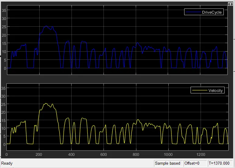
UDDS DRIVE CYCLE(1370secs):
The scope result shows the actual drive cycle velocity (blue) and vehicle output velocity(yellow), the output velocity after simulation is following the given drive cycle.
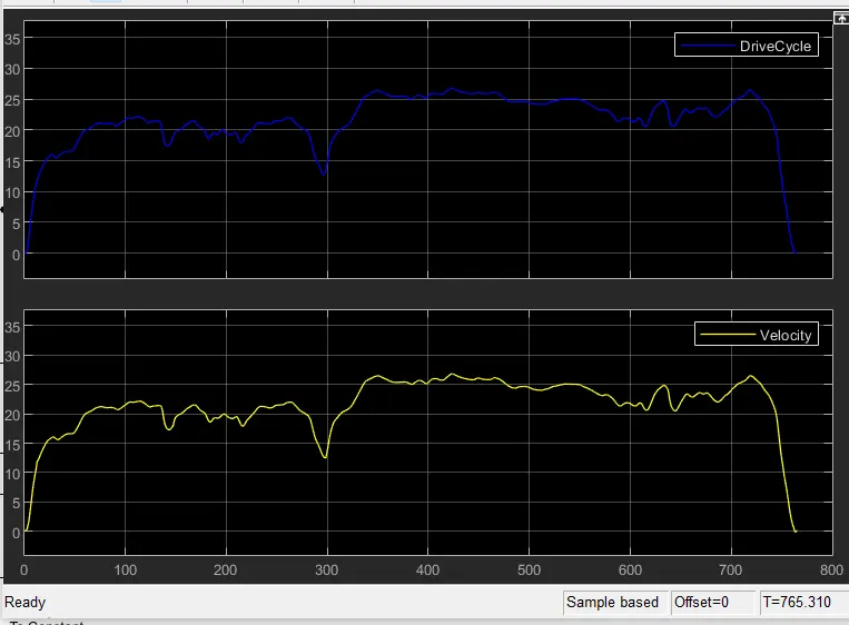
HWFET DRIVE CYCLE (800 secs):
The scope result shows the actual drive cycle velocity (blue) and vehicle output velocity(yellow), the output velocity after simulation is following the given drive cycle.
a. Tabulate the fuel economy numbers (kmpl) for UDDS and HWFET cycle. Compare these numbers with the baseline numbers for conventional vehicle model from Project 1.
Fuel economy number of drive cycle is calculated and tabulated using the formula
kmpl = Veh_Dist(end)/(Eng_Fuel_Consump(end)/1000/rho_petrol);    % Fuel economy [kmpl]

% Display Fuel Economy of the Cycle
fprintf('n fuel economy of drive cycle = %2.2f kmpl ',kmpl)
fuel economy number of P1 hybrid vehicle
UDDS fuel economy:

HWFET fuel economy:

fuel economy of HWFET cycle is more than UDDS cycle, because UDDS cycle have more loss and it have large number for braking and acceleration commands. HWFET cycle have less engine idle time and less accelerationa and braking.
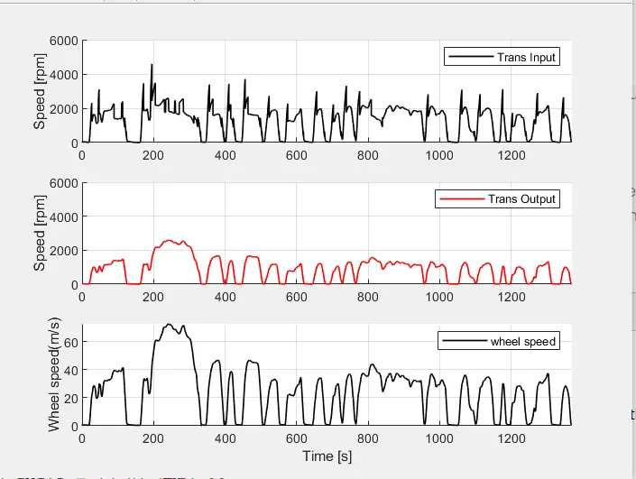
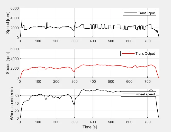
b. Plot the time trace for engine, transmission input, transmission output and wheel speed on one plot.
The time trace is plotted for the transmission input ,transmission output and wheel speed.
Transmission output is lower than the transmission input in both the cycle.
UDDS cycle time trace:
HWFET cycle time trace:
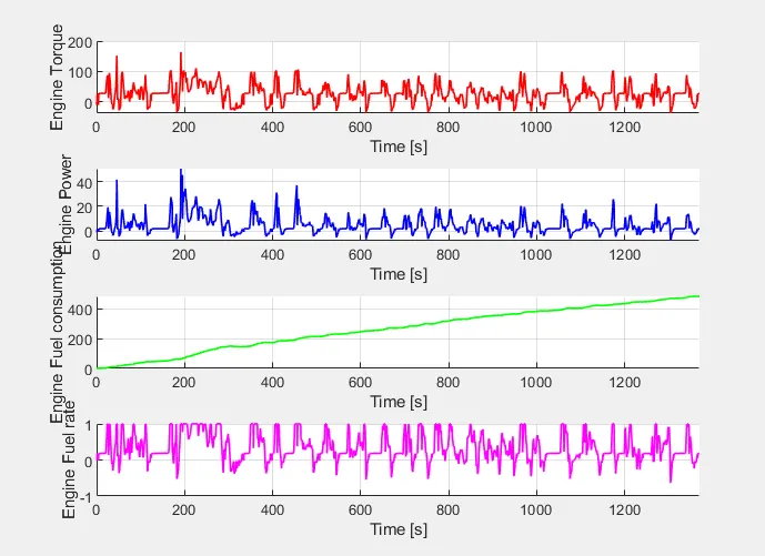
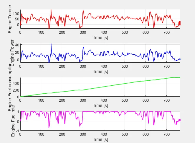
c. Plot engine torque, engine power, fuel rate and fuel consumption using subplots.
engine torque, engine power, fuel rate and fuel consumption are plotted for both cycles using the subplots.
for udds cycle engine fuel rate is changes frequently whereas in HWFET cycle engine fuel rate is maintained and at some points and engine torque and power more than the udds drive cycle.
UDDS cycle engine parameter plots:
HWFET cycle engine parameters plot:
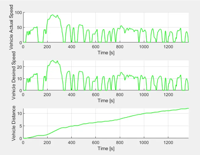
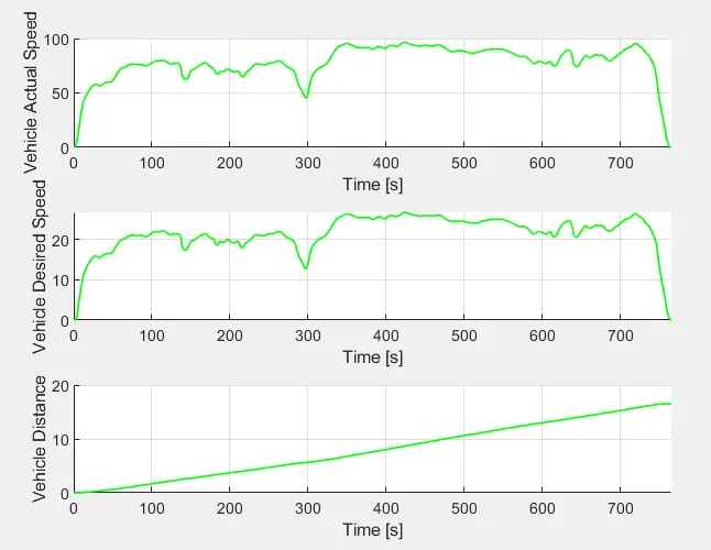
d. Plot accelerator and brake pedal, gear command, vehicle desired and actual speed, vehicle distance using subplots.
accelerator and brake pedal, gear command are plotted using the subplots.
UDDS cycle pedal % and gear plots:
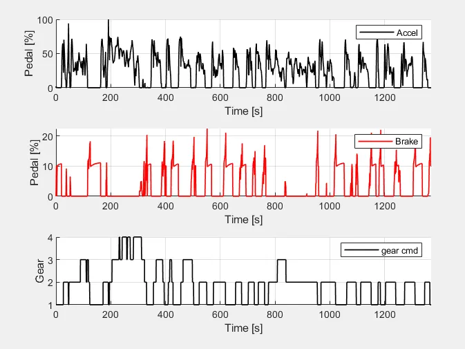
In udds cycle we able see that the gear changes are more than hwfet cycle,and brake pedal is more frequently applied equal to the acceleration pedal.
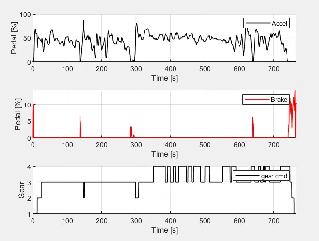
HWFET cycle pedal % and gear plots:
In HWFET cycle brake pedal is rarely applied and gear command changes is less compared to udds cycle.
vehicle desired and actual speed, vehicle distance are plotted using subplots the actual and desired speed is maintained equally for both the drive cycles More distance is travelled by the HWFET cycle than the UDDS cycle.
UDDS cycle vehicle actual and desire speed and vehicle distance plot:
HWFET cycle vehicle actual and desire speed and vehicle distance plot:
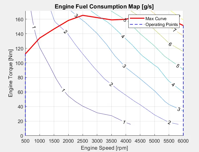
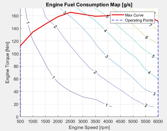
e. Plot the engine operating points on the engine fuel map.
Engine operating points are plotted for both the drive cycle using the plot,set and contour commands
UDDS cycle engine operating points plot:
HWFET cycle engine operating points plot:
f. Plot motor speed, torque, motor input power using subplots.
UDDS cycle motor parameters plot:
HWFET cycle motor parameters plot:
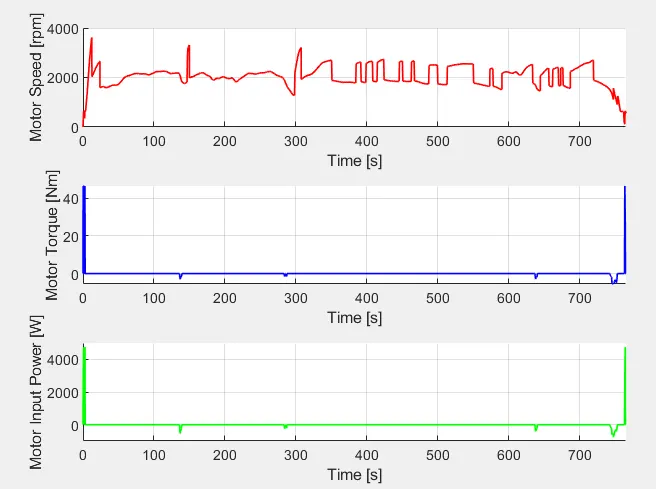
The motor torque,speed and power is less for HWFET cycle the because in highway cycle there is less use of start and stop system and not require the motor torque requirement much. In UDDS cycle, traffic is more the use of start and stop and idle position is more so it uses the motor at regular intervals so the motor power of UDDS cycle changes frequently throughout the cycle.
g. Plot pack voltage, current and SoC using subplots.
Using the equivalent circuit model the terrminal voltage and SOC is estimated
UDDS cycle battery pack parameters plot:
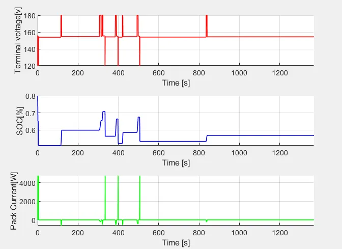
The soc is changes according to the motor electric power,it will charge and discharge and maintain at the 0.5% of the battery pack.
HWFET cycle battery pack parameters plot:
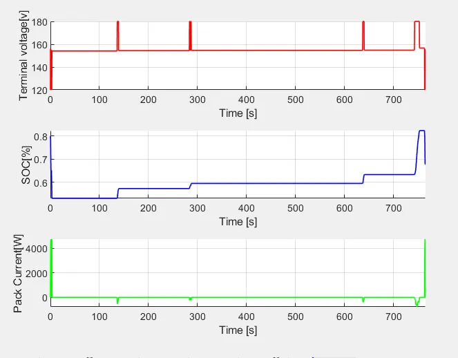
In HWFET cycle, we can get the see the soc is decreased because it takes more power in acceleration and because of less regenerative braking.
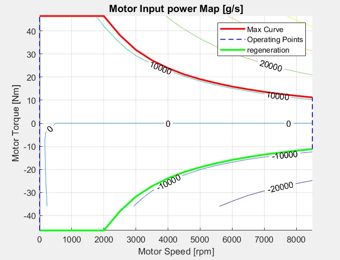
h. Plot the motor operating points on the motor input power map, with the motor max motoring and generating torque curves.
motor operating points are plotted on the motor input power map, with the motor max motoring and generating torque curves using the plot,set and contour commands.
UDDS cycle motor operating points plot:
HWFET cycle motor operating points plot:
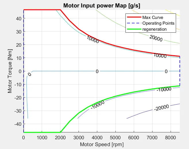
Here, we can see the region of torque and speed where the motor is operate within this range.
COMPARISION OF FUEL ECONOMY NUMBERS:
Project 1:
Fuel economy number of conventional vehicle
UDDS Cycle: 16.35 kmpl
HWFET Cycle: 18.32 kmpl
Project 2:
Fuel economy number of P1 Hybrid vehicle
UDDS Cycle: 19.48 kmpl
HWFET Cycle: 21.04 kmpl
Here we can see that fuel economy of the P1 hybrid vehicle is more than the fuel economy numbers of the conventional vehicle.
City driving cycle is less than the Highway cycle because of the brake pedal and idle positions are less in the highway cycle in both the conventional and hybrid vehicle.
The fuel economy of the P1 hybrid vehicle is more because of implementing the electric motor between the engine and transmission in project 2,which is not available in conventional vehicle. It will reduce the loss by wasting power during the traffic by idle start and stop provision by the motor in the P1 hybrid where the conventional vehicle this is not available so it is giving the less fuel economy numbers.
CONCLUSION:
The forward energy based fuel consumption model of a P1 hybrid vehicle is model using the MATLAB scripts and SIMULINK model based on the conventional vehicle model of project 1.
- Fuel economy numbers (kmpl) for UDDS and HWFET cycle are compared with the baseline numbers for conventional vehicle model from Project 1.
- time trace for engine, transmission input, transmission output and wheel speed are plotted as one plot.
- engine torque, engine power, fuel rate and fuel consumption are plotted using subplots.
- accelerator and brake pedal, gear command, vehicle desired and actual speed, vehicle distance are plotted using subplots.
- engine operating points on the engine fuel map are plotted and motor speed, torque, motor input power are plotted using subplots.
- pack voltage, current and SoC are plotted using subplots.
- motor operating points on the motor input power map, with the motor max motoring and generating torque curves are plotted.
The vehicle behaviour throughout the cycle is studied and the characteristics are plotted for both the UDDS and HWFET drive cycles and the fuel economy number of P1 hybrid vehicle is compared with the conventional vehicle.
REFERENCES:
https://x-engineer.org/mild-hybrid-electric-vehicles-mhev-types/
https://www.researchgate.net/figure/Zero-order-equivalent-circuit_fig4_321143431