Week 4.1 - Genetic Algorithm

1. The algorithm begins by creating a random initial population.

2. The algorithm then creates a sequence of new populations. At each step, the algorithm uses the individuals in the current generation to create the next population. To create the new population, the algorithm performs the following steps:

   1. Scores each member of the current population by computing its fitness value. These values are called the raw fitness scores.

   2. Scales the raw fitness scores to convert them into a more usable range of values. These scaled values are called expectation values.

   3. Selects members, called parents, based on their expectation.

   4. Some of the individuals in the current population that have lower fitness are chosen as elite. These elite individuals are passed to the next population.

   5. Produces children from the parents. Children are produced either by making random changes to a single parent—mutation—or by combining the vector entries of a pair of parents—crossover.

   6. Replaces the current population with the children to form the next generation.

3. The algorithm stops when one of the stopping criteria is met like maxgeneration,maxtime,functional tolerance

4. The algorithm takes modified steps for linear and integer constraints.

5. The algorithm is further modified for nonlinear constraints.

GA Syntax:

We used the below syntax of ga in this project.

STEP 1:

CODE OF STALAGMITE FUNCTION

function [S] = stalagmite_func(input_vector)

x = input_vector(1);
y = input_vector(2);

f1x = (sin((5.1*pi*x)+0.5))^6;
f1y = (sin((5.1*pi*y)+0.5))^6;
f2x = exp(-4*log(2)*((x-0.0667)^2/0.64));
f2y = exp(-4*log(2)*((y-0.0667)^2/0.64));

S = -(f1x*f1y*f2x*f2y);

end

EXPLANATION:

The function S is created with function name stalagmite_func

x and y values are inputs and that are given

the formulas are splitted into terms and combined and defined for function S

Negative symbol is used in formula to get the max values.

STEP 2:

CODE FOR OPTIMIZATION OF STALAGMITE FUNCTION AND FIND THE GLOBAL MAXIMA

%Study of statistical behaviours of GA using stalagmite example function
clear all
close all
clc

%stalagmite mathematical model
x = linspace(0,0.6,150);
y = linspace(0,0.6,150);
no_of_its = 50;

%create 2d mesh
[xx yy] = meshgrid(x,y); 

%evaluating stalagmite function
for i=1:length(xx)
    for j=1:length(yy)

        input_vector(1) = xx(i,j);
        input_vector(2) = yy(i,j);
        f(i,j) = stalagmite_func(input_vector);
    end
end

tic
%statistical behavior 1 - unbounded limits

for i = 1:no_of_its
    [inputs,fopt(i)] = ga(@stalagmite_func,2);
    xopt(i)= inputs(1);
    yopt(i) = inputs(2);
end

study1_time = toc

figure(1)
subplot(2,1,1)
hold on 
surfc(xx,yy,-f)
shading interp
plot3(xopt,yopt,-fopt,'marker','o','MarkerSize',5,'MarkerFaceColor','b')
xlabel('xvalue');
ylabel('yvalue');
title('unbounded limits');
subplot(2,1,2)
plot(-fopt);
xlabel('iterations');
ylabel('maximum function');

tic
%statistical behavior 2 with upper and lower bounds

for i = 1:no_of_its
    [inputs,fopt(i)] = ga(@stalagmite_func,2,[],[],[],[],[0,0],[1,1]);
    xopt(i)= inputs(1);
    yopt(i) = inputs(2);
end
study2_time = toc

figure(2)
subplot(2,1,1)
hold on 
surfc(xx,yy,-f)
shading interp
plot3(xopt,yopt,-fopt,'marker','o','MarkerSize',5,'MarkerFaceColor','r')
xlabel('xvalue');
ylabel('yvalue');
title('bounded limits');
subplot(2,1,2)
plot(-fopt);
xlabel('iterations');
ylabel('maximum function');


tic
%statistical behavior 3 with increase in population size
options = optimoptions('ga');
options = optimoptions(options,'PopulationSize',170);

for i = 1:no_of_its
    [inputs,fopt(i)] = ga(@stalagmite_func,2,[],[],[],[],[0,0],[1,1],[],[],options);
    xopt(i)= inputs(1);
    yopt(i) = inputs(2);
end
study3_time = toc

figure(3)
subplot(2,1,1)
hold on 
surfc(xx,yy,-f)
shading interp
plot3(xopt,yopt,-fopt,'marker','o','MarkerSize',5,'MarkerFaceColor','r')
xlabel('xvalue');
ylabel('yvalue');
title('increase in population size option');
subplot(2,1,2)
plot(-fopt);
xlabel('iterations');
ylabel('maximum function');


%end

EXPLANATION:

step 1:

Inputs for stalagmite model x and y are given using linspace command and no of iterations are given.

step 2:

2d array of inputs are created using meshgrid command.

Step 3:

creating of stalagmite model for the inputs by calling the stalagmite_func using for loop

STUDY OF STATISTICAL BEHAVIOURS OF GA:

STUDY 1:

UNDERSTANDING OF STATISTICAL BEHAVIOURS OF GA USING UNBOUNDED LIMITS

tic
%statistical behavior 1 - unbounded limits

for i = 1:no_of_its
[inputs,fopt(i)] = ga(@stalagmite_func,2);
xopt(i)= inputs(1);
yopt(i) = inputs(2);
end

study1_time = toc

EXPLANATION OF STUDY 1:

Using for loop run the ga algorithm for no of iteration(50) to get the fopt(global max value) and optimum inputs xopt and yopt for that optimimum result.

using tic toc command study time is calculated.

In

figure (1)

using subplot comand 3 segments are plotted

1. stalagmited model function

surfc(xx,yy,-f)

-F is given to plot the downward stalagmite and to get the max value of F.

2. optimum values

plot3(xopt,yopt,-fopt,'marker','o','MarkerSize',5,'MarkerFaceColor','b')

3. max function(-fopt) vs iterations

plot(-fopt);

plots of study 1:

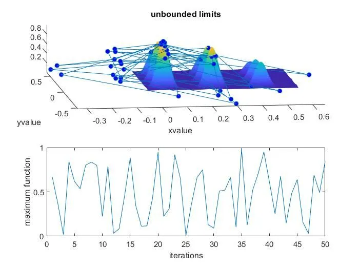
The above plot shows the behaviour of ga using unbounded limits.

STUDY 2:

UNDERSTANDING OF STATISTICAL BEHAVIOURS OF GA USING LOWER AND UPPER BOUNDS:

tic
%statistical behavior 2 with upper and lower bounds

for i = 1:no_of_its
[inputs,fopt(i)] = ga(@stalagmite_func,2,[],[],[],[],[0,0],[1,1]);
xopt(i)= inputs(1);
yopt(i) = inputs(2);
end
study2_time = toc

EXPLANATION OF STUDY 2:

Here the major change is in the syntax of GA ,we are using the lower and upper bound limits in the syntar for further optimization.

Using for loop run the ga algorithm for no of iteration(50) to get the fopt(global max value) and optimum inputs xopt and yopt for that optimimum result.

using tic toc command study time 2 is calculated.

In

figure (2)

using subplot comand 3 segments are plotted

1. stalagmited model function

surfc(xx,yy,-f)

2. optimum values

plot3(xopt,yopt,-fopt,'marker','o','MarkerSize',5,'MarkerFaceColor','b')

3. max function(-fopt) vs iterations

plot(-fopt);

plots of study 2:

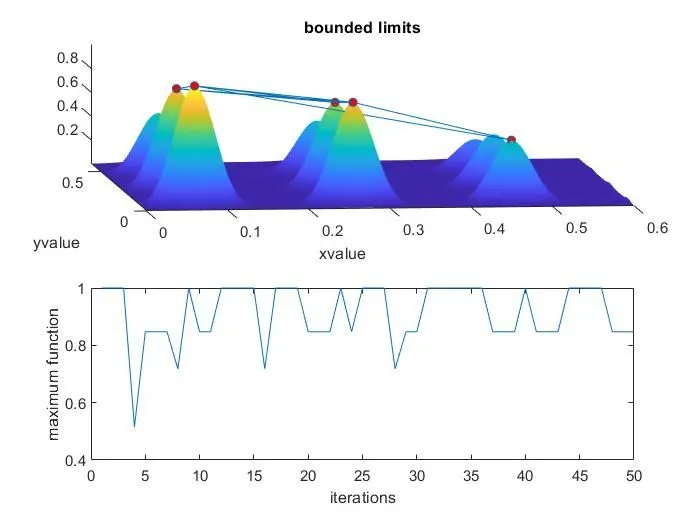
the above plots show the behaviour of ga using limited bounds,here we can see the change in graphs and able to get the somewhat converged optimum values.

STUDY 3:

UNDERSTANDING OF STATISTICAL BEHAVIOURS OF GA USING OPTIONS (INCREASING THE POPULATION SIZE):

tic
%statistical behavior 3 with increase in population size
options = optimoptions('ga');
options = optimoptions(options,'PopulationSize',170);

for i = 1:no_of_its
[inputs,fopt(i)] = ga(@stalagmite_func,2,[],[],[],[],[0,0],[1,1],[],[],options);
xopt(i)= inputs(1);
yopt(i) = inputs(2);
end
study3_time = toc

EXPLANATION OF STUDY 3:

Here the major change is in the syntax of GA ,we are using the lower and upper bound limits in the syntar for further optimization.

Using for loop run the ga algorithm for no of iteration(50) to get the fopt(global max value) and optimum inputs xopt and yopt for that optimimum result.

using tic toc command study time 3 is calculated.

In

figure (3)

using subplot comand 3 segments are plotted

1. stalagmited model function

surfc(xx,yy,-f)

2. optimum values

plot3(xopt,yopt,-fopt,'marker','o','MarkerSize',5,'MarkerFaceColor','b')

3. max function(-fopt) vs iterations

plot(-fopt);

plots of study 3:

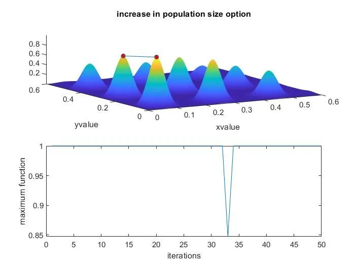
Above plot shows the maximum functions for all the iterations except 1 iteration,it is clearly shown that by using optimoptions we can get the optimized result,here we can able to get the optimum value for repeated iterations.

under a set of prioritized criteria or constraints the statisfactory solution is found.

ERRORS WHILE PROGRAMMING:

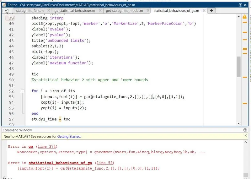
in ga syntax forget to add the nil value brackets for linear equalities.

the correct syntax is given below

x = ga(fun,nvars,A,b,Aeq,beq,lb,ub) defines a set of lower and upper bounds on the design variables, x, so that a solution is found in the range lb ≤ x ≤ ub. (Set Aeq=[] and beq=[] if no linear equalities exist.)

CONCLUSION:

The matlab code is written for optimise the stalagmite function using ga algorithm

genetic algorithm concept and syntax are explained and using the varioys syntax of ga the statistical behaviours of ga are calculated and plotted and also study time for the various study behaviours are calculated.

global maxima of the function are found and plotted.

REFERENCES:

https://towardsdatascience.com/introduction-to-genetic-algorithms-including-example-code-e396e98d8bf3#:~:text=A%20genetic%20algorithm%20is%20a,offspring%20of%20the%20next%20generation.

https://in.mathworks.com/help/gads/how-the-genetic-algorithm-works.html