Development of a forward energy-based fuel consumption model of a P1 hybrid vehicle
PROJECT 2
Development of a forward energy-based fuel consumption model of a P1 hybrid vehicle
Objective of the project:-
The main goal of this project is to understand the functionality of a P1 hybrid and be able to model it.
Honda Insight motor and battery are considered for this project. Data is taken from ADVISOR data base developed by NREL, USA. Data provided in the project files.
Task:-
The task of this project is to quantify the improvement in fuel economy numbers for the hybrid vehicle (kmpl), compared to the conventional vehicle, on the urban cycle (UDDS) and highway cycle (HWFET). Also, to analyze and understand the vehicle operating points in terms of engine and motor speed, torque, transmission speeds, pedal positions, gear, distance traveled, battery voltage, current, SoC etc.
P1 Hybrid Vehicle:-
The P1 architecture, with the electric machine connected directly to the crankshaft, is the solution adopted by Honda on their first generation Integrated Motor Assist (IMA) technology. The electric motor functions as a generator, during vehicle deceleration, as an engine starter, and as a motor (to assist the engine) during vehicle accelerations.
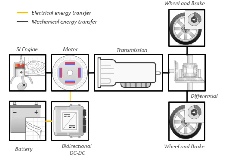
One of the biggest advantage of this solution is that the electric motor can provide higher torque than the BiSG, since there is no belt limitation (due to slip). However, since there is no speed / torque ratio between the electric machine and crankshaft, the torque requirements on the electric motor can be quite demanding.
Two examples of P1 architectures are:
- Honda Insight Hybrid
- Mercedes Benz S400 Bluehybrid 2010
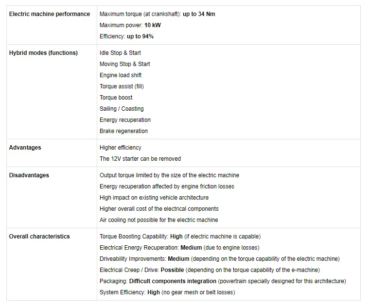
For example, the main characteristics of the crankshaft-mounted electric machine for hybrid Honda Insight are summarized in the table below.
VEHICLE MODELLING USING MATLAB:-
%%%%%%%%%%%%%%%%%%%%%%%%%%%%%%%%%%%%%%%%%%%%%%%%%%%%%%%%%%%%%%%%%%%%%
%% Hybrid Drives Development
% Project 2 - P1 Hybrid Vehicle Model
% By - Altrin Rijo

% Description:

%% Initialization File
% Initialization file for loading the variables for the Conventional vehicle simulation model

%% Vehicle Parameters
M = 1500;       % Vehicle weight [kg]
Cr = 0.015;     % Rolling resistance coefficient
Rw = 0.35;      % Rolling radius [m]
Cd = 0.33;      % Drag coefficient
Af = 2;         % Frontal area [m2]
rhoa = 1.225;   % Air density [kg/m3]
Vwind = 0;      % Wind velocity [kmph]
g = 9.81;       % Gravitational acceleration [m/s2]
theta = 0;      % Slope [deg]
myu_road_tire = 1; % Coefficient of friction between tire - road interface

%% Powertrain Parameters
FDR = 3.73;                         % Final Drive Ratio / Diff Ratio
DiffEff = 0.99;                     % Differential efficiency (assumed independent of operating conditions)

NumGear = 4;                        % Number of gears in transmission
TransGear = [1:NumGear];            % Transmission Gears
TransRatio = [3.06, 1.62, 1, 0.7];  % Corresponding Transmission ratios
TransEff = 0.90;                    % Transmission efficiency (assumed independent of operating conditions)

TC_SR = [0, .5, .6, .7, .8, .87, .92, .94, .96, .97, 1];   % Torque Converter Speed Ratio (Matlab default) -> TurbSpd/PumpSpd
TC_TR = [2.232, 1.5462, 1.4058, 1.2746, 1.1528, 1.0732, 1.0192, 1, 1, 1, 1];   % Torque Converter Torque Ratio (Matlab default) -> TurbTrq/PumpTrq
TC_Cf = 1e-4 * [.72558, .66322, .63463, .59042, .51331, .4144, .29287, .22444, .12186, .04386, 0]; % Torque Converter Capacity Factor (Matlab default) -> PumpTrq/PumpSpd^2 [Nm/rpm^2]

load Vehicle_Data/Engine_data_1_9L_Saturn_95kW
load Vehicle_Data/Trans_Shift_map
load Vehicle_Data/EM_Honda_Insight_10kW
load Vehicle_Data/ESS_NiMH6


ESS_init_soc = 0.8;
ESS_soc_max = 0.9;
ESS_soc_min = 0.6;


%% Driver Parameters
Kp = 10;                    % P gain for driver PI model
Ki = 1;                     % I gain for driver PI model
Drive_Cycle_Select = 2;     % Drive cycle selection

% Drive cycle values in m/s

if Drive_Cycle_Select == 1
    load DriveCycles/UDDS;

elseif Drive_Cycle_Select == 2
    load DriveCycles/HWFET;

elseif Drive_Cycle_Select == 3
    load DriveCycles/FTP;

elseif Drive_Cycle_Select == 4
    load DriveCycles/US06;

elseif Drive_Cycle_Select == 5
    load DriveCycles/NEDC;

elseif Drive_Cycle_Select == 6
    load DriveCycles/WLTP;

end

time_end = cyc_time(end);
vel_end = cyc_vel(end);
In this above matlab script, all the input parameters which are mainly required for a conventional vehicle are discussed. As we can see, Vehicle parameters, Powertrain parameters, Driver parameters including the Drive cycles are also scripted. We can choose different drive cycles by changing the varialbe "Drive_Cycle_Select = 1; % Drive cycle selection"
| Drive cycle Variable | Drive Cycle selected |
| 1 | UDDS |
| 2 | HWFET |
| 3 | FTP |
| 4 | US06 |
| 5 | NEDC |
| 6 | WLTP |
So according to our driving conditions we can choose our own drive cycle easily. Here in this project the all the important vehicle parameters are detailedly explained for UDDS and HWFET drive cycles.
SIMULINK MODEL:-
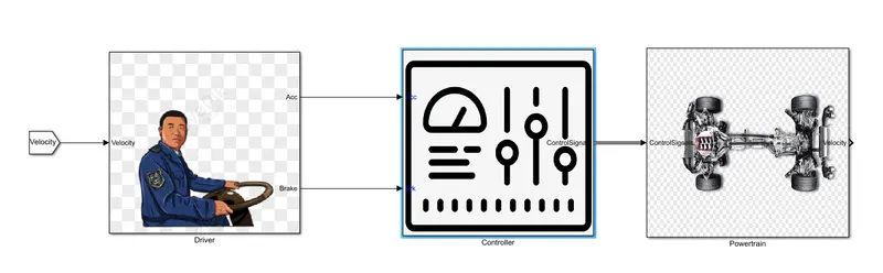
These are the three important subsystems or blocks, which are used to model the P1 Hybrid vehicle. The three important blocks are Driver block, Controller block and the powertrain block. We will discuss the blocks one by one below:-
1)Driver Block:-
When you open the driver block,the following models are present:-
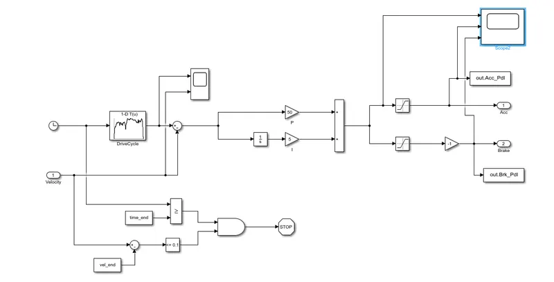
A driver model is a mathematical model which replicates the. functionality of a driver( controlling , monitoring and stabilizing a vehicle )during various maneuvers.It is modeled using a ‘Driver’ block, which is a basic PI controller that generates accelerator and brake pedal outputs to match the desired and actual vehicle speeds. In this we use drive cycles fro the based on these results of fuel consumption and emissions the vehicle gets certified and it also forms a basis of uniform asessment. It is based on time, velocity then its all integrate and creates output accelration pedal and brake pedal.
2) Controller Block:-
The controller block has been modelled as follows:-
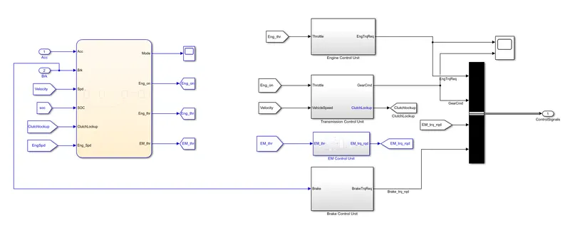
The controller block, mainly consists of the following blocks.
a) Mode controller
b) Engine control unit
c) Transmission Control unit
d) Electric Machine control unit
e) Brake control unit
a) Mode controller:-
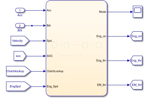
When you open this Mode controller chart,
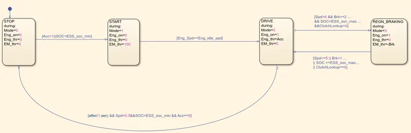
This state flow diagram represents the four modes of an vehicle . The first block is for the Starting condition of an engine ,2nd Block represent the start condition of the engine ,3rd Block gives a condition for the drive mode and the 4th block is the conditions for the regenerative braking.Now the each modes can be explained here as follows:-
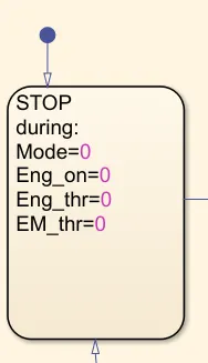
This is the first block of our state flow and it represents the idle condition of the vehicle. And we have described the mode as zero for the vehicle in idle condition.
Since the vehicle is in idle state, the Engine ON condition is 0, The Engine throttle and the Electric motor throttle will be Zero.
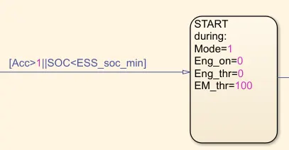
This is our second block of the state flow, which represents the starting condition of the vehicle. And hence the mode is represented as 1, and certain rules or defined for converting from the first condition to the second condition. ie.,When the acceleration is greater than one or when the is SOC is lesser than the minimum state-of-charge value then the stop condition will change to the start condition. And during the start condition the engine will be still in the OFF condition the engine throttle will be Zero but the engine motor throttle will be in maximum.
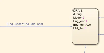
The drive mode will be our third state and its mentioned as Mode 2 for our state flow. And this condition will gets activated when the Engine speed is Greater or equal to the Engine idle speed .When this condition gets satisfied the engine will be ON and it is given as 1 , and the engine throttle will be there and that is the given input acceleration and the engine motor throttle will be zero.
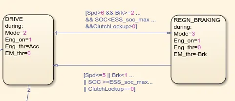
The fourth state represents the regenerative braking and it is given as Mode 3. When that top condition is satisfied it will change from the mode 3 to mode 2 and when the bottom condition is satisfied then it will again change from the mode 3 to Mode 2 ie., from regenerative braking to the drive mode. The first condition is satisfied when the speed is in 6th gear and the brake is applied and also the SOC is lesser than the maximum state-of-charge value and the clutch lock up will be there. If this condition is satisfied, then the regenerative braking condition is activated.
But when the second condition is satisfied that is when the speed is lesser than or equal to the fifth gear , or when the brake is not applied, or when the SOC is greater than or equal to the maximum SOC or when the clutchlockup is zero then the mode 3 that is regenerative braking mode is again gets converted back to the drive mode.
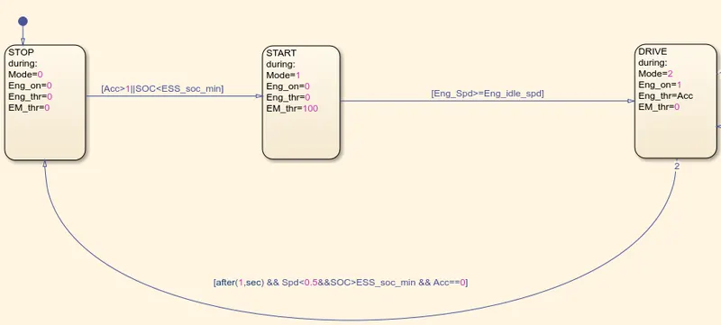
And also the drive mode will be changed back to the stop mode when the last condition is satisfied, that is after 1 second when the speed value is less than 0.5 and the SOC is lesser than its minimum value and when the acceleration is zero (ie., No throttling) the vehicle will be again converted back to the stop mode.
And finally with the help of 'Symbols pane' option, the input and the output parameters are defined for the control logic.
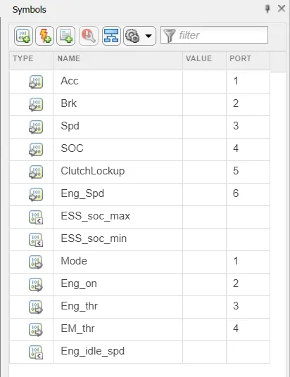
This is the working of the created state flow.
b) Engine Control unit:-
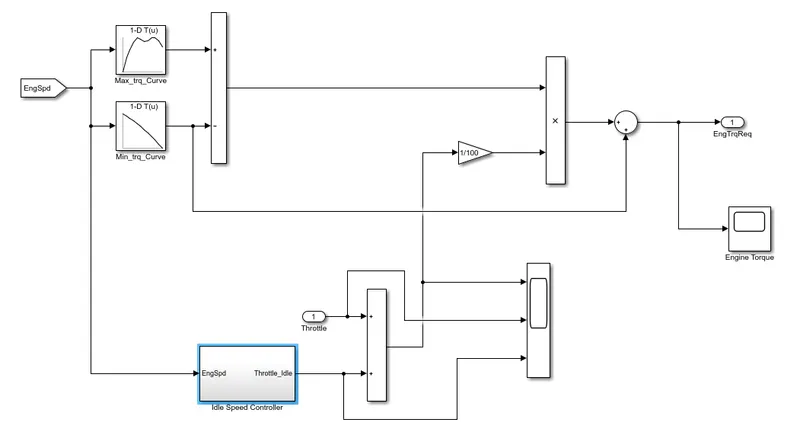
For the engine control unit, the accleration is given as the input. In this engine control unit all the necessary parameters which are required for the running performance of the engine is modelled. And hence for the given engine speed the Engine torque and idle speed can also be found out with the help of this engine control block.And hence the required throttle can be found out with in the model. And with the help of the scope block, all the all the parameters like Engine torque, idle speed and the throttle performances can be analysed graphically.
Since it is a P1 hybrid vehicle, duriing the very slow moving rate, the engine can be run as idle, when it is ran by the motor. So an Idle speed controller block is attached with the engine cooontrol unit.
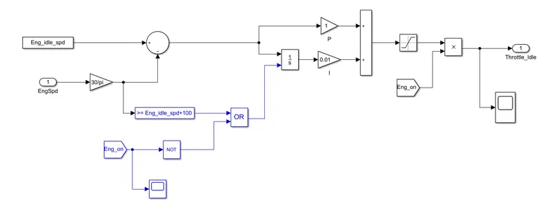
So even when the Engine is in Off state, ie., in idle state, the vehicle can be run with the help of the motor.
c) Transmission Control unit:-
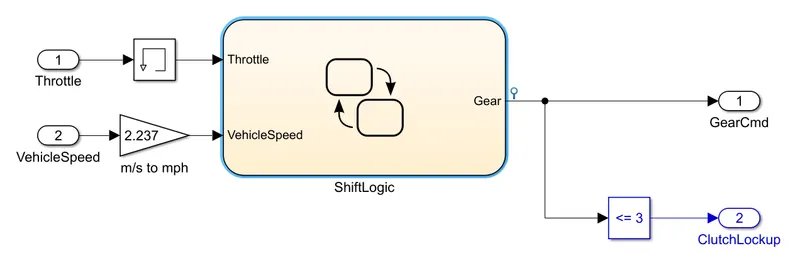
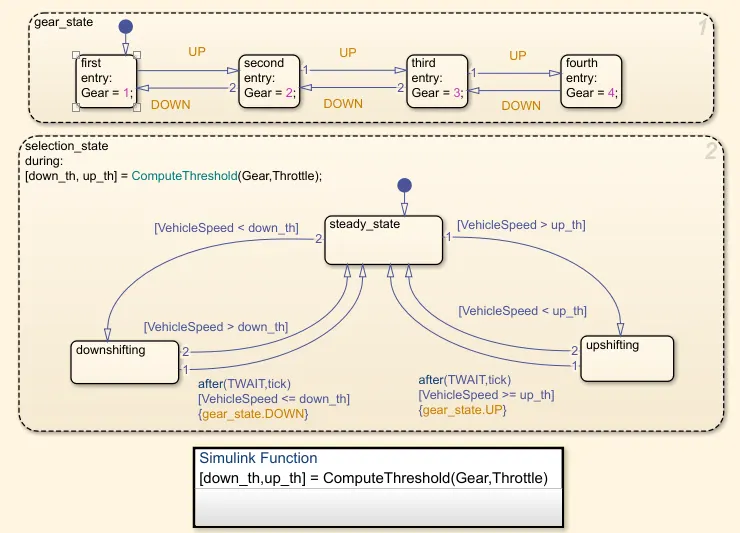
Hear the gear shifting Logics are done with the help of matlab scripting. The vehicle speed is given as the input for the gear shifting logic and depending upon the speed variation the respective gear is selected and is chosen to run the vehicle .As we can see in the second image the gear shifting logic is provided and the different speeds are analysed and depending upon the speed the correct gear is selected.It will automatically shift to the lower gears when the speed reduces to the optimum value which is defined in the shift logic.The out put signal from this block is also used to modify the powertrain parameters.
The clutchlockup condition is also defined here.That is, when the engine runs with less than a third gear, the clutch will get engaged and the vehicle can run with the help of the motor and engine combined.
c) Electric Machine Control unit:-
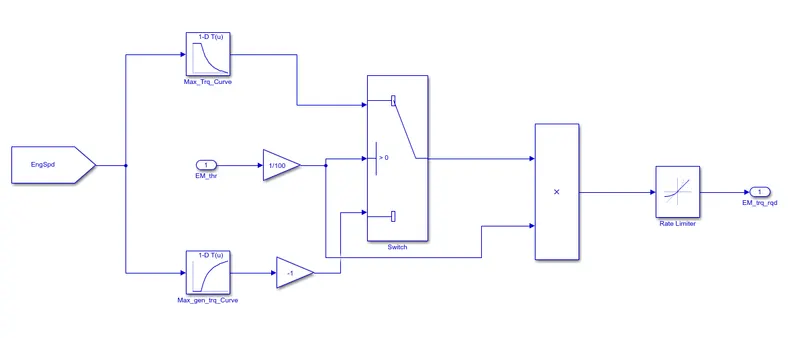
The Electric motor parameters are defined here. That is for the given motor throttle, the torque required for the motor can be calculated. And it is defined in between the maximum and minimum torque values.
d) Brake Control unit:-
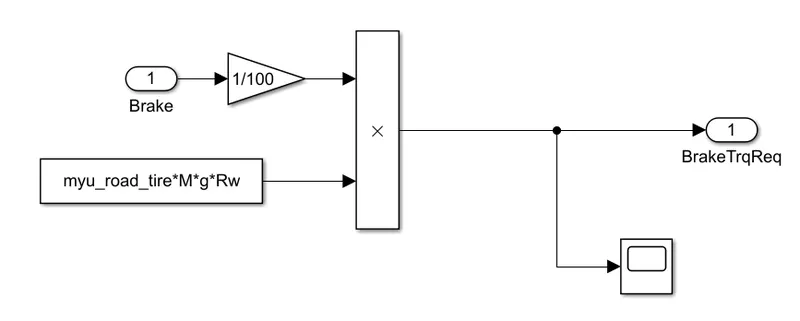
In this block, the brake torque is calculated as per the vehicle drive cycles defined.
And finally all the outputs of these 4 units are fed into the Powertrain block, to calculate and visualize all the powertrain parameters.
3) Powertrain Block:-
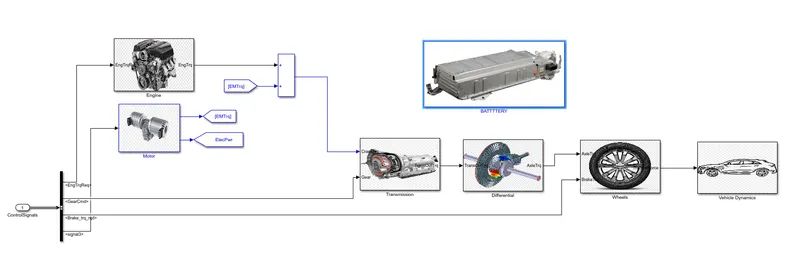
Inside the powertrain subsystem we will have the following units:-
a) Engine unit
b) Motor unit
c) Transmission unit
d) Differential unit
e) Wheels
f) Vehicle Dynamics.
g) Battery
Let us discuss the each blocks one by one.
a) Engine unit:-
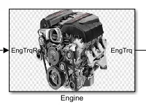
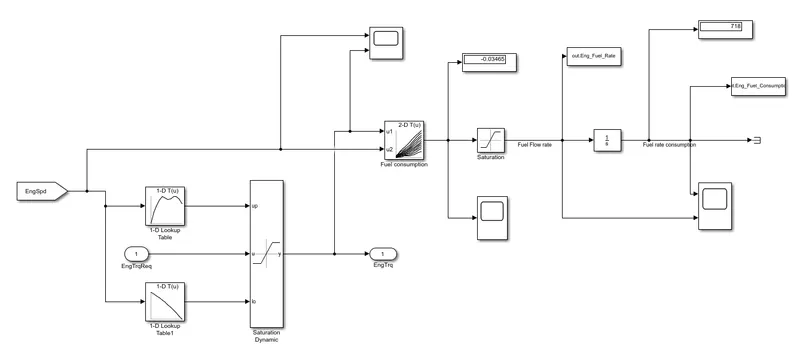
The engine speed is given as the input for the engine block and for that engine speed given, the fuel consumption and the fuel flow rate can be calculated in this engine block. The maximum torque and the minimum torque are taken up into a 1D lookup table and they are fed into the saturation dynamic block so that both that the optimum values are chosen by the saturation dynamic block and we will obtain the final engine torque value.
And then the final engine torque and engine speed is fed into the fuel consumption 2D lookup table for those consumption again a saturation block is chosen to to obtain the minimum and maximum limits and the output of the saturation lord will give you the fuel flow rate when that fuel flow rate this integrated with the help of the integrator block actual fuel rate consumption can be found out and then the signal is terminated.
Two 'To workspace' blocks are used to get the engine fuel rate and the engine fuel consumption to the matlab workspace with the help of two workspace block. This is the working of the engine block Model.
b) Motor Unit:-
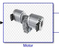
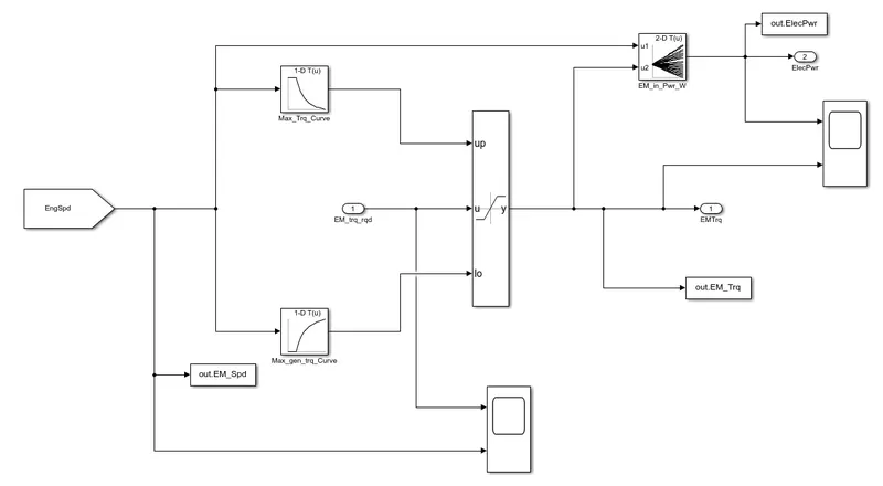
The electric motor torque which is derived from the EM unit is fed as the input for the Motor unit block. Also the minimum and the maximum torque of the motor is defined using the 1D look up tables and the proper value is taken with the help of the 'Saturated Dynamic Block'. The output from this block gives us the torque required for the electric motor. Also, to find the required Electric power , the engine speed and the and the Electric motor torque values are fed into the 2D look up table.
The final value of Electric power and the Torque of electric motor will be taken back to our matlab file with the help of the 'To Workspace block'
c) Transmission Unit:-
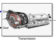
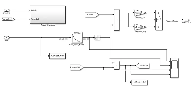
The Engine torque and the Electric motor torque are added up and that is provided as the input for the transmission unit.
The transmission model comprises from the given gear input and for the given gear inputs, the gear ratios are calculated and finally the transmission output speed and the transmission out put torque are calculated. The transmission output signal is taken as the next input for the vehicle dynamics block.
The another important sub block used is the 'Torque converter block'. When you open the torque converter block, the following blocks will get displayed.
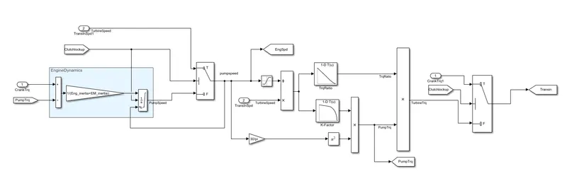
A torque converter is a type of fluid coupling that transfers rotating power from a prime mover, like an internal combustion engine, to a rotating driven load. In a vehicle with an automatic transmission, the torque converter connects the power source to the load. It is usually located between the engine's flexplate and the transmission. The equivalent location in a manual transmission would be the mechanical clutch.
The main characteristic of a torque converter is its ability to increase torque when the output rotational speed is so low that it allows the fluid coming off the curved vanes of the turbine to be deflected off the stator while it is locked against its one-way clutch, thus providing the equivalent of a reduction gear. This is a feature beyond that of the simple fluid coupling, which can match rotational speed but does not multiply torque and thus reduces power.
And here in our model, The pump torque and turbine torque are calculated for the given speed. The Clutchlockup is used to stop the working of the torque converter, when the vehicle is running only with the help of the motor. And hence, for the obtained pumb and turbine speed and torque, the input is provided to the differential unit.
d) Differential Unit:-
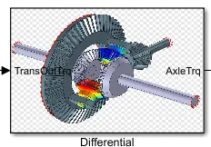
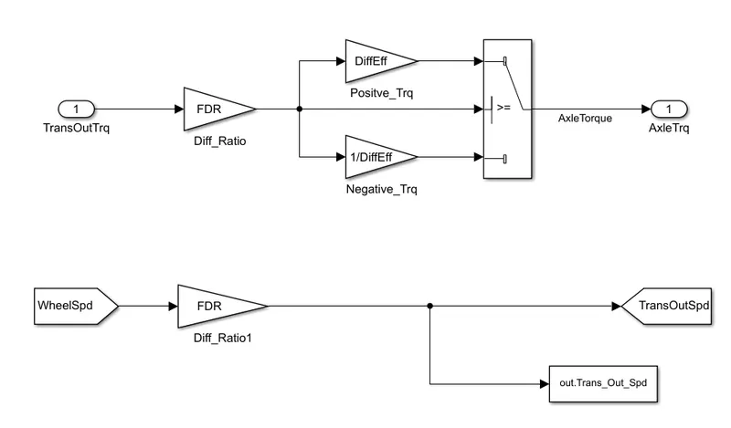
In this differential block, for the given transmission output torque, the axle torque is calculated. A switch block is connected in between the positive and negative torque gain blocks, so that only the positive torque is taken into the consideration and for that positive torque , the axle torque is calculated.
e) Wheels:-
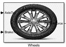
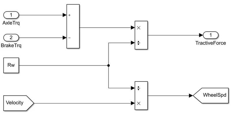
Here in this wheel block, For the provided Axle and brake torques, the tractive force and for the obtained velocity, the wheel speed is also calculated.The brake torque from the control model is subtracted from the Axle torque and divides from the rolling radius to determine the Tractive force. And hence we can obtain the Tractive force and the wheel speed from this above model.
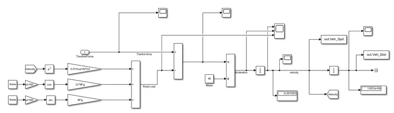
f) Vehicle Dynamics:-
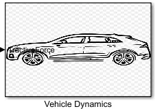
The vehicle movement is described by the longitudinal forces equation:
where:
Ft [N] – traction force
Fi [N] – inertial force
Fs [N] – road slope force
Fr [N] – road load force
Fa [N] – aerodynamic drag force
The traction force can be regarded a a “positive” force, trying to move the vehicle forward. All the other forces, are resistant, “negative” forces which are opposing motion, trying to slow down the vehicle.
Here,
The inertial (resistant) force [N] is given by the equation:
The road slope (resistant) force [N] is given by the equation:
The road load (resistant) force [N] is given by the equation:
The aerodynamic drag (resistant) force [N] is given by the equation:
Replacing (4) in (1) and rearranging the terms, gives:
By integrating equation (10) we obtain the vehicle speed [m/s]:
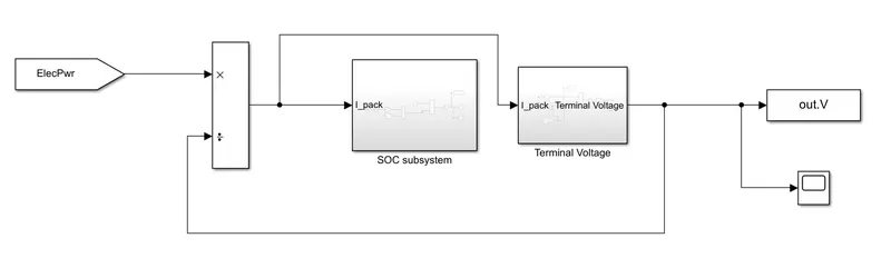
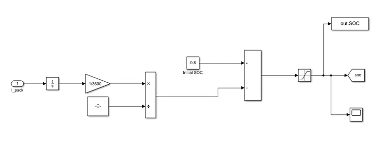
In this blocks, the given Pack current is loaded in the 'constant block' and with the help of respective blocks it is subtracted with the initial SOC. (here the initial soc is taken as 0.8). Then the 'Saturation block' is used to limit the SOC values from 0 to 1 (ie., from 0% to 100%).
The peak current is integrated and we will get the values in coulumbs and when it is again didivided by 3600 we will get the current values in Amphere.
And finally, 'To workspace' blocks are used to fetch the values of SOC & Pack current to our matlab script.
And the 'SOC' values are taken using the 'From Block' and is fed as the input for the Terminal voltage circuit.
TERMINAL VOLTAGE SUBSYSTEM:-
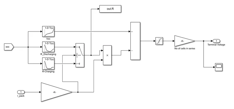
The SOC is given as the input for the Voc, Discharge Resistance and for the Charging Internal resistance.
And hence with the help of the Switch block, The Discharge and charge internal resistance are compared with the Pack current and the product is obtained.
With the help of 'To workspace' block, the Resistance values are fetched to the matlab script.
And finallly, the saturation block is used to limit the voltages between the Minimum voltage and Maximum voltages.
And then , when it is multiplied with the number of cells connected in series, we will get the Terminal voltage value.
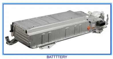
This is the complete woking of the battery unit.
OUTPUT DISCUSSIONS:-
1) FOR UDDS DRIVE CYCLE:-
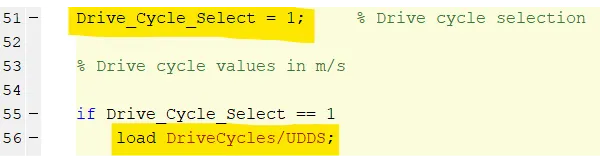
In the drive cycle selection, choose 1 for the UDDS drive cycle
a) The UDDS drive cycle Vs the velocity:-
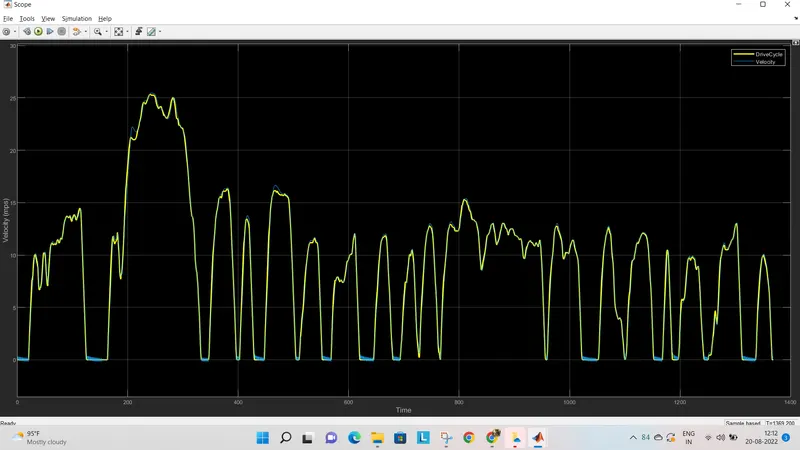
From the driver block we will get the curve for the UDDS drive cycle which we have implemented in the matlab script as we can clearly see that the velocity is higher in between the values of time 200 to 300 seconds so we will discuss with this maximum velocity for our upcoming graphs and we can verify whether our script and model is behaves depending upon the speed variations provided in our UDDS drive cycle. We can also see that the velociity curve and the drive cycle curve matches toogether.And also we can witness that the velocity is matching with the drive cycle.
b)Transmission input vs Transmission Output vs Wheel speed plots:-
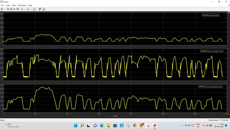
These plots represent the Wheel speed of the vehicle with respect to the provided output value of the transmission. The transmission input value looks quite similar to the drive cycle provided and for that input the transmission output is generated. The transmission out put is then fed back to the wheels of the vehicle and we can clearly see that, whenever the transout is higher, the wheel speed is also getting higher plot values.
c) Plots between Engine torque vs Fuel Flow rate vs Fuel Consumption:-
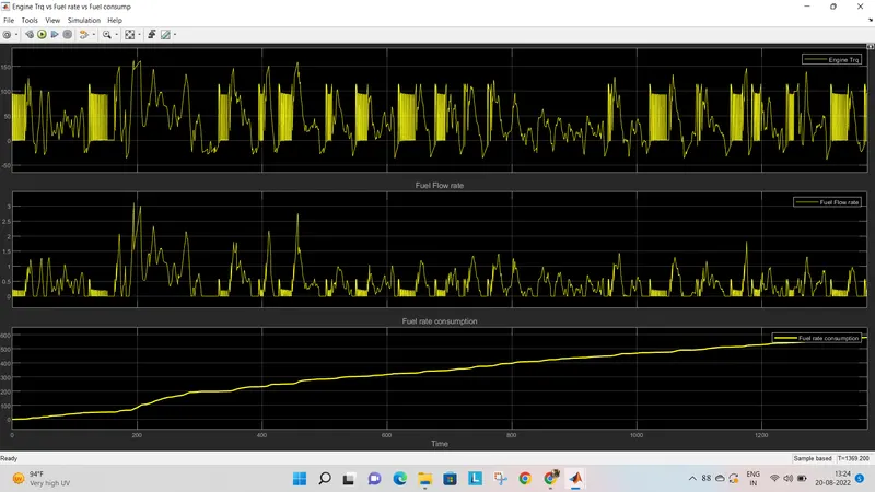
In this plots the first graph represents the engine torque, the second graph represent the fuel flow rate and the third graph represent the fuel rate consumption of the engine. We can clearly see that according to the engine torque, the fuel consumption value will vary and we can also see that wherever the engine torque is higher we can visualise a higher amount of peak in the fuel flow rate and while looking into the third graph we can visualise that the fuel rate consumption is increasing for the run Period of the vehicle for the provided engine torque.
d) Plots between Brake pedal and the Gear command for the given accleration:-
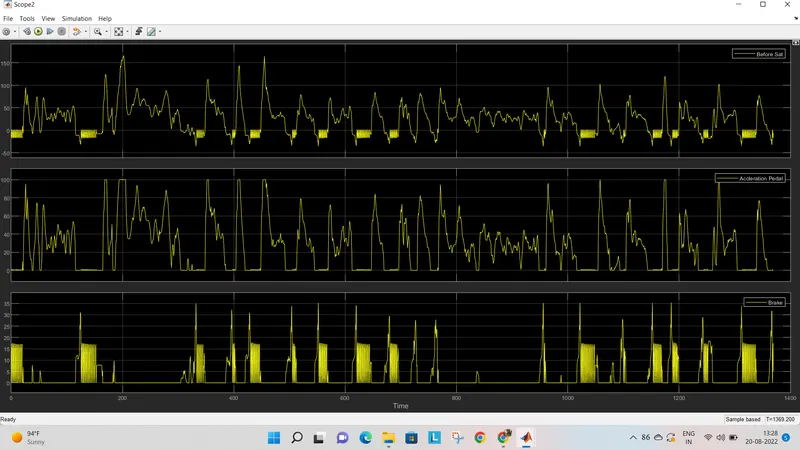
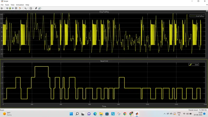
Here then we compare the second and third plot, it is very clear that whenever there is zero acceleration pedal value the brake value is higher( ie., Brake is applied) and similarly when our the acceleration Rises to the peak value then the brake value tends to zero ,which represent whenever there is acceleration given to the vehicle, no break is applied to the vehicle and when the acceleration becomes zero that is when the driver takes off his left from the acceleration the brake is applied to the way and that value of brake can be clearly visualised in the third plot.
And the last plot represent the Gear command value. When the accleraton pedal is applied, higher speed will be provided for the vehicle and hence the gear command value will reached the value 4 (ie., 4th gear). Similarly whenever the accleration pedal is reduced, the value of gear also comes down and it will be in the 1st gear whenwver the accleration pedal value reaches zero.
Distance covered by the vehicle:-
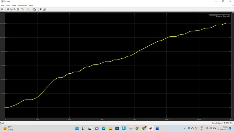
This plot represent the distance covered by the vehicle for the 1400 seconds, which was provided as the stimuation time. And here we can see that the distance is getting varied from 0 to 1200m .
e) Plots of Motor Torque vs Motor Speed vs Motor Power:-
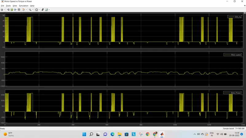
This plot represents the motor parameters. The first plot represent the Motor torque, the second one represents the Motor speed and the third plot represents the Motor power. Here we can see that, for the higher torque values, the speed of the motor will be lesser and viceversa. And we know that the torque and the power are directlyy propotional to each other, and hence we can also see that the power of the motor is getting increased for the provided torque values in the same manner.
f) Plots of Pack Voltage, Current and SOC:-
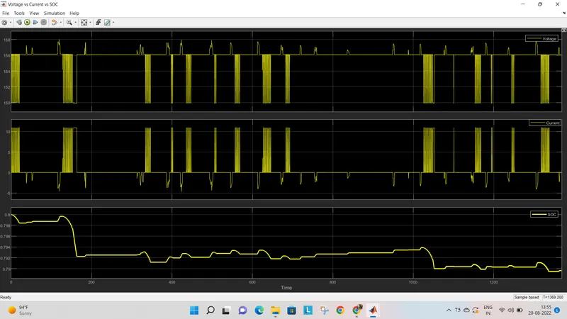
Here the first plot represent the voltage, and the second plot represent the current and the third plot represent the SOC value of the battery. As we all know that the voltage and current are inversely proportional ,we can see that point clearly in the first two plots whenever there is a rise in the voltage value we can see that dip in the current plot.
And the third plot is representing the SOC of the battery. As we can clearly see that the value of SOC is following the path of voltage and current. Whenever the current is higher the value of SOC is reducing. And we can also see some of the sudden rise in the SOC plot, which represents the charging state of the battery . This is seen whenevr the current value goes below zero that is whenever the motor is running in the opposite direction the current value goes less than 0 which represents the Regenerative braking of the battery.
OUTPUT DISCUSSIONS:-
2) FOR HWFET DRIVE CYCLE:-
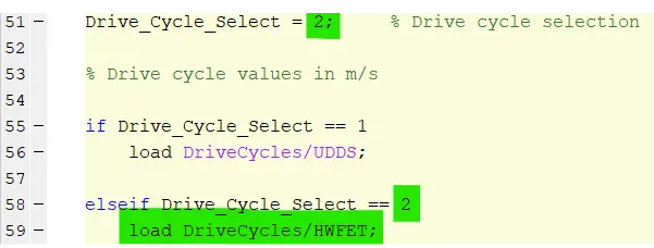
In the drive cycle selection, choose 2 for the HWFET drive cycle in the initial matlab script file as follows:-
a) Drive cycle plot:-
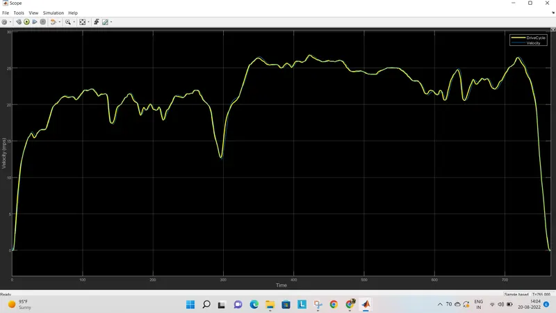
This plot represent the HWFET drive cycle. We can see that the velocity value is matching along with the drive cycle.
b)Transmission input vs Transmission Output vs Wheel speed plots:-
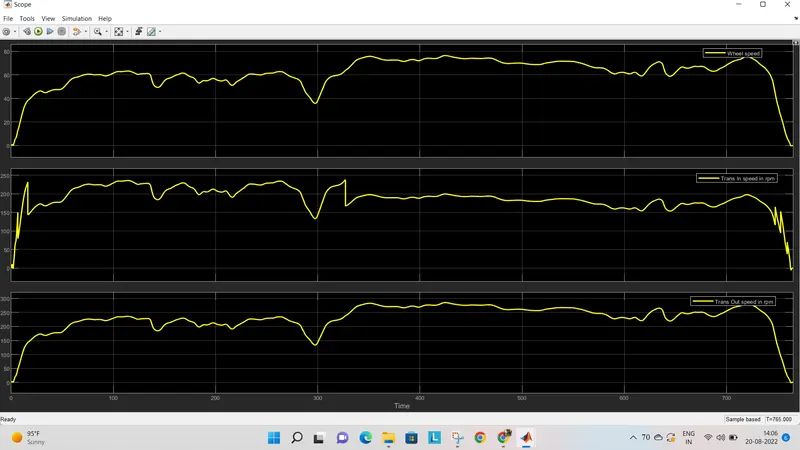
These plots represent the Wheel speed of the vehicle with respect to the provided output value of the transmission. The transmission input value looks quite similar to the drive cycle provided and for that input the transmission output is generated. The transmission out put is then fed back to the wheels of the vehicle and we can clearly see that, whenever the transout is higher, the wheel speed is also getting higher plot values.
c) Plots between Engine torque vs Fuel Flow rate vs Fuel Consumption:-
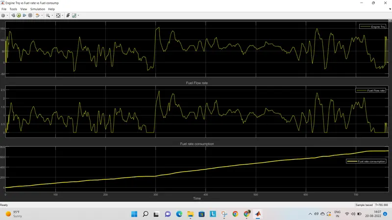
In this plots the first graph represents the engine torque, the second graph represent the fuel flow rate and the third graph represent the fuel rate consumption of the engine. We can clearly see that according to the engine torque, the fuel consumption value will vary and we can also see that wherever the engine torque is higher we can visualise a higher amount of peak in the fuel flow rate and while looking into the third graph we can visualise that the fuel rate consumption is increasing for the run Period of the vehicle for the provided engine torque.
d) Plots between Brake pedal and the Gear command for the given accleration:-
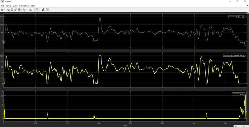
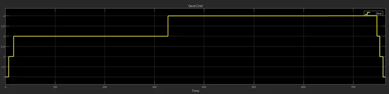
These plots represent the Accleration, Brake pedal and Gear command for the HWFET drive cycle. We can see clearly that Whenever the value of accleration pedal is higher, we can see zero values peaak fro the brake (ie., No brake is applied). And similarly , when the accleration pedal value is higher we can see that the Gear command of the vehicle is also higher (ie., Vehicle is running in the 4th gear) and vice versa.
e) Plots of Motor Torque vs Motor Speed vs Motor Power:-
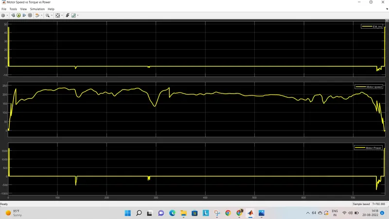
These plots represent the motor torque, Motor speed and the Motor power respectively. Here as we can see , when the motor torque increases, the power of the motor will also increases. Similarly when we compare the motor torque and the motor speed, it willl be a inversely propotional ie., for higher motor torque the speed will be lesser and viceversa. And here as most of the times, the vehicle will be in the running mode and hence there is no work for the motor and since the motor torque and motor power values are zero at most of the running period of the vehicle.
f) Plots of Pack Voltage, Current and SOC:-
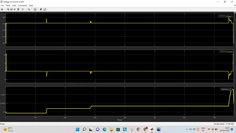
Since it is a Highway Drive condition, Most of the times, the vehicle will be in the high speed and hence it will be run with the help of the fuel. And so, the motor is very rarely engaged. And we can witness that the SOC value of the battery is in constant for most of the time and Whenver there is a negative current value, we can see the rise in the SOC plot, which represent the Regenerative braking.
POST PROCESSING MATLAB SCRIPT:-
%%%%%%%%%%%%%%%%%%%%%%%%%%%%%%%%%%%%%%%%%%%%%%%%%%%%%%%%%%%%%%%%%%%%%
%% Skill-Lync -> Hybrid Drives Development
% Project 2 - P1 Hybrid Vehicle model
% By - Altrin Rijo

% Description:
% The following file is to used with the Initialization file and Simulink
% results for post-processing of the data.
% The file is incomplete, has some examples of how the data is imported
% into a readable format, data analysis and plotting examples.
% Based on the project task, use commands in a similar format as given
% below, to analyse the data and generate required plots.
% You can change variable names if desired

%% Post-Processing File
%  File for post-processing the Conventional vehicle simulation model data

%% Renaming variables
Time = out.tout;
Acc_Pdl = out.Acc_Pdl;          % Accelerator pedal [%]
Brk_Pdl = out.Brk_Pdl;          % Brake pedal [%]
Gear_Cmd = out.Gear_Cmd;        % Transmission gear
Trans_In_Spd = out.Trans_In_Spd*30/pi;  % Transmission input speed [rpm]
Trans_Out_Spd = out.Trans_Out_Spd*30/pi;% Transmission output speed [rpm]
Eng_Trq = out.Eng_Trq;          % Engine brake torque [Nm]
Eng_Spd = out.Eng_Spd*30/pi;    % Engine speed [rpm]
Eng_Fuel_Consump = out.Eng_Fuel_Consumption;    % Engine fuel consumption [g]
Veh_Dist = out.Veh_Dist/1000;   % Distance traveled by vehicle [km]
Veh_Spd = out.Veh_Spd*18/5;     % Vehicle speed [kmph]
motor_power=out.ElecPwr;
motor_trq=out.EM_Trq;
motor_speed=out.EM_Spd;
Final_SOC=out.SOC;
Term_volt=out.Term_Voltage;
Resistance=out.R;

%% Data Analysis
Eng_Pwr = Eng_Spd*pi/30*Eng_Trq/1000;   % Engine brake power [kW]
rho_petrol = 0.7197;                    % Density of petrol [kg/L]
kmpl = Veh_Dist(end)/(Eng_Fuel_Consump(end)/1000/rho_petrol);    % Fuel economy [kmpl]

%% Plotting vehicle characteristics time trace
figure()
subplot(3,1,1)
hold on
grid on
plot(Time, Acc_Pdl, 'linewidth', 1, 'Color', 'black');
plot(Time, Brk_Pdl, 'linewidth', 1, 'Color', 'red');
ylabel('Pedal [%]')
xlim([0, Time(end)]);
legend('Accel','Brake');
subplot(3,1,2)
hold on
grid on
plot(Time, Trans_In_Spd, 'linewidth', 1, 'Color', 'black');
plot(Time, Trans_Out_Spd, 'linewidth', 1, 'Color', 'red');
ylabel('Speed [rpm]')
xlim([0, Time(end)]);
ylim([0, 6000]);
legend('Trans Input','Trans Output');
subplot(3,1,3)
hold on
grid on
plot(Time, Gear_Cmd, 'linewidth', 1, 'Color', 'black');
xlim([0, Time(end)]);
xlabel('Time [s]');
ylabel('Gear');

%% Plotting engine operating points on engine fuel map
figure('Name','Engine Operating Points');
hold on
grid on
title('Engine Operating Points','fontsize',12);
p1=plot(Eng_map_spd*30/pi,Eng_max_trq,'linewidth',2,'color','r');
p2=line([Eng_map_spd(end)*30/pi Eng_map_spd(end)*30/pi],[0 Eng_max_trq(end)]);
set(p2,'linewidth',1,'linestyle','--','color','k');
p3=line([Eng_map_spd(1)*30/pi Eng_map_spd(1)*30/pi],[0 Eng_max_trq(1)]);
set(p3,'linewidth',1,'linestyle','--','color','k');
[c,h] = contour(Eng_map_spd'*30/pi,Eng_map_trq,Eng_fuel_map');
clabel(c,h);
xlabel('Engine Speed [rpm]');
ylabel('Engine Torque [Nm]');
title('Engine Fuel Consumption Map [g/s]');
p4 = plot(Eng_Spd,Eng_Trq,'.','color','k');
legend([p1 p4],{'Max Curve','Operating Points'});
axis([Eng_map_spd(1)*30/pi Eng_map_spd(end)*30/pi 0 Eng_map_trq(end)]);
OUTPUTS:-
1) FOR HWFET DRIVE CYCLE:-
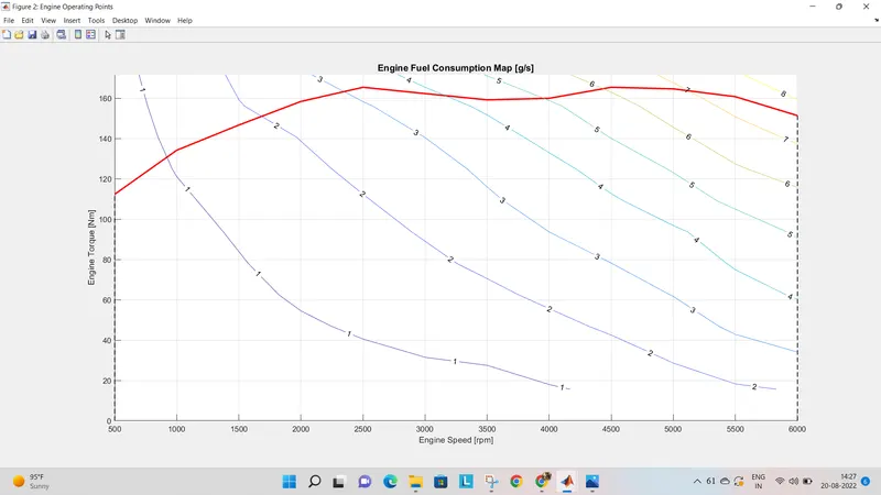
Engine operating points on Engine fuel map:-
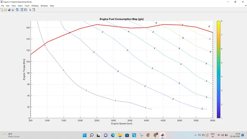
This plot represent the engine fuel consumption for the UDDS drive cycle.Typical fuel consumption map of a engine. The dashed red line represents the maximum torque that the engine can provide at a given rpm. The green line represents one possible, constant power output (which is proportional to the product of rpm and torque).
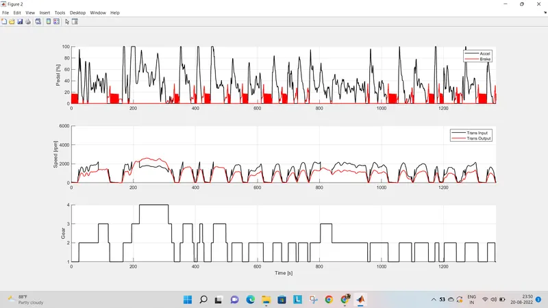
In this graph the plots for the acceleration pedal and the brake pedal are plotted. When we compared these plots to the previous plot that is with our UDDS drive cycle. that acceleration is higher in between the time range of 200 to 300 seconds again when we look into the graph of acceleration pedal and brake pedal we can experience the same heights in the acceleration padel between the period of 200 to 300th seconds and when the vehicle is accelerated between these time period we can see the brake pedal the value remains ZERO.And hence its very clear that the brake pedal values are zero, whenever there is a accleration. (ie., our vehicle is in running mode). Similarly you can see that the gear values are changing for various speeds.
2) FOR HWFET DRIVE CYCLE:-
Engine operating points on Engine fuel map:-
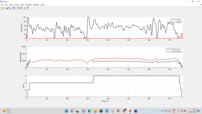
These plots represent the Accleration, Brake pedal and Gear command for the HWFET drive cycle. We can see clearly that Whenever the value of accleration pedal is higher, we can see zero values peaak fro the brake (ie., No brake is applied). And similarly , when the accleration pedal value is higher we can see that the Gear command of the vehicle is also higher (ie., Vehicle is running in the 4th gear) and vice versa.
FUEL ECONOMY COMPARISON:-
FOR UDDS:- FOR HWFET:-

| FUEL CONSUMPTION VALUES:- | UDDS | HWFET |
| PROJECT 1 ( CONVENTIONAL VEHICLE MODEL) | 11.26 kmpl | 15.23 kmpl |
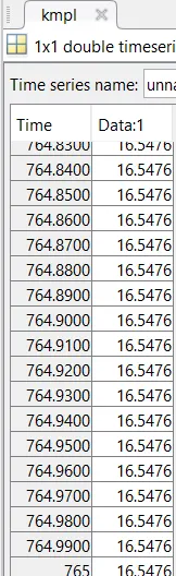
| PROJECT 2 ( HYBRID VEHICLE MODEL) | 14.85 kmpl | 16.54 kmpl |
As we can see the comparision, the Fuel consumption values are better for the hybrid vehicle in both the UDDS and HWFET drive cycles.
******************************END*****************************************
NOTE:- THE .m & .slx FILES ARE ATTACHED WITH THE ANSWER BOX