Project 2:-Principal component analysis, K-Means Clustering & Hierarchical Clustering.

Project Brief:

International humanitarian NGO have been able to raise around $ 120 million.Now the CEO of the NGO call us to choose how to use this money strategically and effectively. The significant issues that comes while making this conclusion are mostly related to choosing the countries that are in the direst need of aid.

Our job is to classify the countries using some socio-economic and health factors that determine the overall development of the country. Then you need to suggest the countries which the CEO needs to focus on the most.

Apply Principal component analysis, K-Means Clustering & Hierarchical Clustering.

#---------------------------------First we Import Important Labreries For our Model.---------------------------------
import numpy as np
import pandas as pd
import matplotlib.pyplot as plt
import seaborn as sns
from sklearn.preprocessing import StandardScaler

from sklearn.decomposition import PCA
from sklearn.decomposition import IncrementalPCA

from sklearn.cluster import KMeans
from scipy.cluster.hierarchy import linkage
from scipy.cluster.hierarchy import dendrogram
from scipy.cluster.hierarchy import cut_tree

%matplotlib inline

---------------------- Data Preprocessing-----------------

#----------------------------------------Importing the file into our model-----------------------------------------

country_data = pd.read_csv("/Users/macbook/Documents/Data Science/Indroduction To Machine learing /Project 2/Country-data.csv")
country_data.head()

#------------------------------------------Data Cleaning Opreation----------------------------------------------
country_data.info()
country_data.describe()

country_data.isnull().sum()      # We cheack for null value in our data
country_data.columns

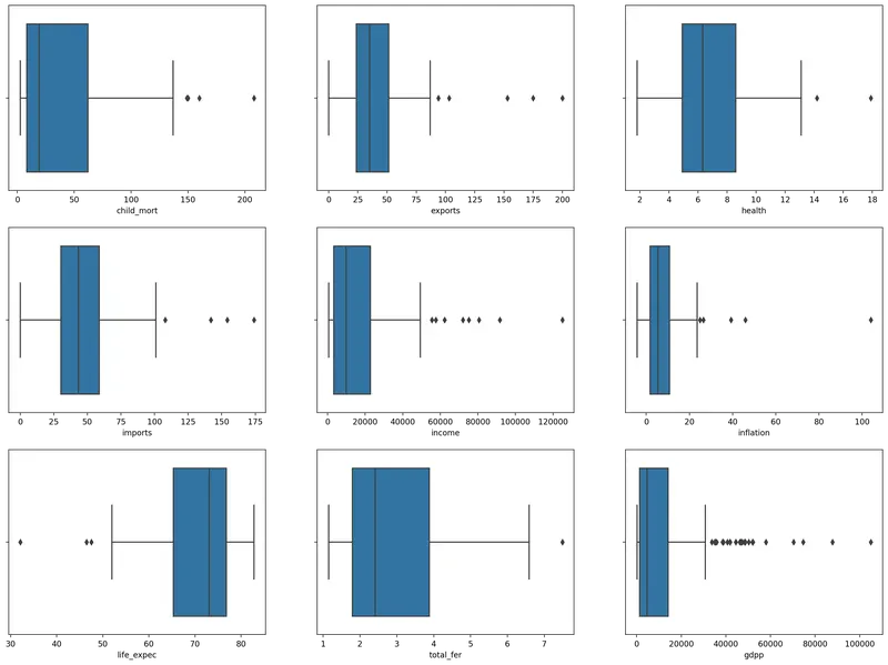
#-------------------------------------------Checking for outliers--------------------------------------

plt.figure(figsize=(20,20), dpi=200)

plt.subplot(4,3,1)
sns.boxplot(x = 'child_mort', data = country_data)

plt.subplot(4,3,2)
sns.boxplot(x = 'exports', data = country_data)

plt.subplot(4,3,3)
sns.boxplot(x = 'health', data = country_data)

plt.subplot(4,3,4)
sns.boxplot(x = 'imports', data = country_data)

plt.subplot(4,3,5)
sns.boxplot(x = 'income', data = country_data)

plt.subplot(4,3,6)
sns.boxplot(x = 'inflation', data = country_data)

plt.subplot(4,3,7)
sns.boxplot(x = 'life_expec', data = country_data)

plt.subplot(4,3,8)
sns.boxplot(x = 'total_fer', data = country_data)

plt.subplot(4,3,9)
sns.boxplot(x = 'gdpp', data = country_data)

# ------------------------------------checking for outliers using the Z-score--------------------------------------

from scipy import stats

z = np.abs(stats.zscore(country_data[['child_mort', 'exports', 'health', 'imports', 'income',
       'inflation', 'life_expec', 'total_fer', 'gdpp']]))
print(z)

print("n")
print("*******************************************************************************")
print("n")

# threshold = 3  # selecting 3 as the threshold to identify outliers
print('Below are the outlier points along with the respective column numbers in the second array')
print("n")
print(np.where(z > 3))

#------------------------------------------ Removing the outliers------------------------------------------------
country_data_outliers_removed = country_data[(z<3).all(axis=1)]
country_data_outliers_removed.head()
print('Shape of dataframe before outlier removal: ' + str(country_data.shape))
print("n")
print('Shape of dataframe after outlier removal: ' + str(country_data_outliers_removed.shape))

#-------------------------------------------Feature And Target Values---------------------------------------
X = country_data_outliers_removed.drop('country',axis =1)  
y = country_data_outliers_removed['country']

#------------------------------------------Now We scale the split-----------------------------------------------------
scaler = StandardScaler()
X_scaled = scaler.fit_transform(X)
X.columns
X_scaled_df = pd.DataFrame(X_scaled,columns=X.columns)
X_scaled_df.head()

#------------------------------------------------Correlation Matrix-----------------------------------------------
plt.figure(figsize = (20,10))       
sns.heatmap(X_scaled_df.corr(),annot = True,cmap="YlGnBu")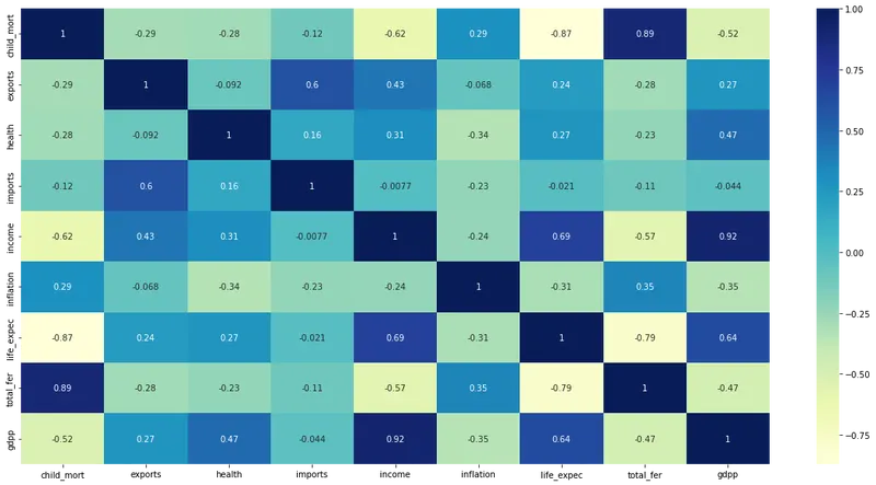

Principal component analysis

#-----------------------------------------------Performing pca-------------------------------------------
pca = PCA(random_state=42)
pca.fit(X_scaled)
pca.components_[0]
pca.explained_variance_ratio_
var_cumu = np.cumsum(pca.explained_variance_ratio_)
var_cumu

fig = plt.figure(figsize=[12,8],dpi=200)
plt.vlines(x=4, ymax=1, ymin=0, colors="r", linestyles="--")
plt.hlines(y=0.95, xmax=30, xmin=0, colors="g", linestyles="--")
plt.plot(var_cumu)
plt.ylabel("Cumulative variance explained")
plt.show()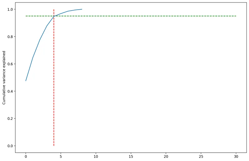

#-------------------------------------------------Performing PCA with 4 components---------------------------------
pca_final = IncrementalPCA(n_components=4)
X_pca_final = pca_final.fit_transform(X_scaled)
print(X.shape)
print(X_pca_final.shape)

# --------------------------------------Plotting the heatmap of the corr matrix--------------------------------------
corrmat = np.corrcoef(X_pca_final.transpose())
plt.figure(figsize=[10,10])
sns.heatmap(corrmat, annot=True)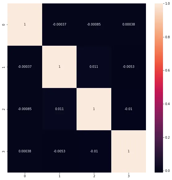

Clustering

1.K - means clustering

# ---------------------------------k-means with some arbitrary k (number of clusters)-------------------------------

kmeans = KMeans(n_clusters=5, max_iter=1000)
kmeans.fit(X_pca_final)
kmeans.labels_

#-------------------------------------------------elbow-curve-----------------------------------------------
ssd = []
range_n_clusters = [2, 3, 4, 5, 6, 7, 8]
for num_clusters in range_n_clusters:
    kmeans = KMeans(n_clusters=num_clusters, max_iter=1000)
    kmeans.fit(X_pca_final)
    
    ssd.append(kmeans.inertia_)
    
# plot the SSDs for each n_clusters
# ssd
plt.plot(ssd)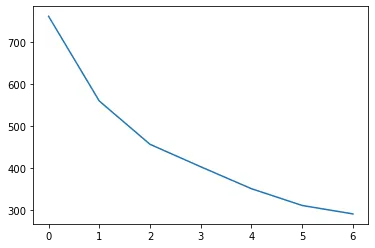

From the elbow method we can say that k = 4 clusters seems to be a good choice

# -------------------------------------------final model with k=3-----------------------------------------
kmeans = KMeans(n_clusters=4, max_iter=1000, random_state=42)
kmeans.fit(X_pca_final)
kmeans.labels_
country_data_outliers_removed['K-Means_Cluster_ID'] = kmeans.labels_

plt.figure(figsize=(8,4),dpi=200)
sns.boxplot(x='K-Means_Cluster_ID', y='gdpp', data=country_data_outliers_removed)

plt.figure(figsize=(8,4),dpi=200)
sns.boxplot(x='K-Means_Cluster_ID', y='income', data=country_data_outliers_removed)

plt.figure(figsize=(8,4),dpi=200)
sns.boxplot(x='K-Means_Cluster_ID', y='child_mort', data=country_data_outliers_removed)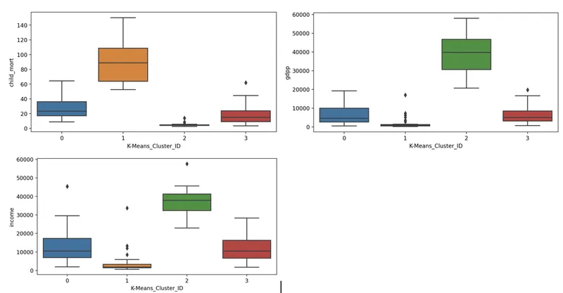

2.Hierarchical Clustering

# ------------------------------------------------single linkage---------------------------------------------
sl_mergings = linkage(X_scaled_df, method="single", metric='euclidean')
dendrogram(sl_mergings)
plt.show()

# ----------------------------------------------complete linkage------------------------------------------------------
cl_mergings = linkage(X_scaled_df, method="complete", metric='euclidean')
dendrogram(cl_mergings)
plt.show()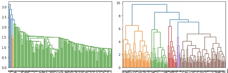

#-----------------------------------plotting sub-plots to analyse the results--------------------------------------

plt.figure(figsize=(20,20), dpi=200)

plt.subplot(3,2,1)
sns.boxplot(x='K-Means_Cluster_ID', y='gdpp', data=country_data_outliers_removed)

plt.subplot(3,2,2)
sns.boxplot(x='Hierarchical_Cluster_labels', y='gdpp', data=country_data_outliers_removed)

plt.subplot(3,2,3)
sns.boxplot(x='K-Means_Cluster_ID', y='child_mort', data=country_data_outliers_removed)

plt.subplot(3,2,4)
sns.boxplot(x='Hierarchical_Cluster_labels', y='child_mort', data=country_data_outliers_removed)

plt.subplot(3,2,5)
sns.boxplot(x='K-Means_Cluster_ID', y='income', data=country_data_outliers_removed)

plt.subplot(3,2,6)
sns.boxplot(x='Hierarchical_Cluster_labels', y='income', data=country_data_outliers_removed)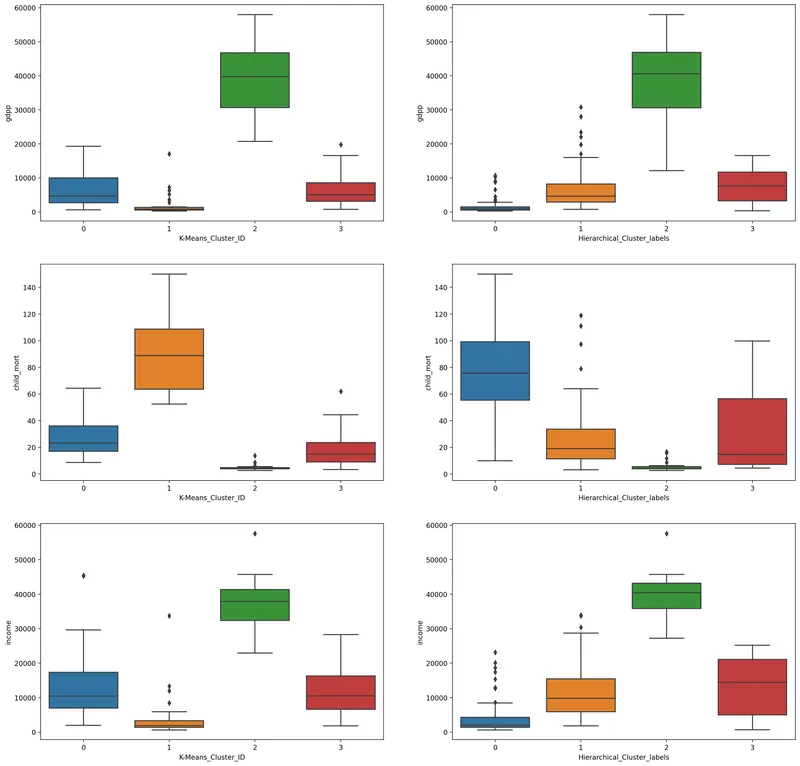

X_pca_final_df = pd.DataFrame(X_pca_final,columns=['PC1','PC2','PC3','PC4'])
X_pca_final_df.head()

X_pca_final_df['K_Means_Cluster_ID'] = kmeans.labels_
X_pca_final_df['Hierarchical_Cluster_Labels'] = cl_cluster_labels
X_pca_final_df.head()

Scatter plot using the first two principal components to observe the cluster distribution

#---------------scatter plot using the first two principal components to observe the cluster distribution-----------

plt.figure(figsize=(12,6),dpi=200)

plt.subplot(1,2,1)
sns.scatterplot(x='PC1',y='PC2',data=X_pca_final_df,hue='K_Means_Cluster_ID')

plt.subplot(1,2,2)
sns.scatterplot(x='PC1',y='PC2',data=X_pca_final_df,hue='Hierarchical_Cluster_Labels')

# -------------------scatter plot using the gdpp, child_mort to observe the cluster distribution--------------------

plt.figure(figsize=(12,6),dpi=200)

plt.subplot(1,2,1)
sns.scatterplot(x='gdpp',y='child_mort',data=country_data_outliers_removed,hue='K-Means_Cluster_ID')

plt.subplot(1,2,2)
sns.scatterplot(x='gdpp',y='child_mort',data=country_data_outliers_removed,hue='Hierarchical_Cluster_labels')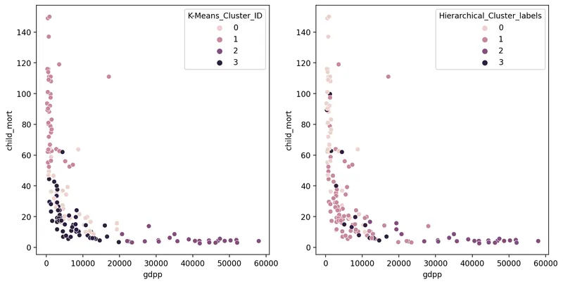

#------------------scatter plot using the gdpp, income to observe the cluster distribution----------------------

plt.figure(figsize=(12,6),dpi=200)

plt.subplot(1,2,1)
sns.scatterplot(x='gdpp',y='income',data=country_data_outliers_removed,hue='K-Means_Cluster_ID')

plt.subplot(1,2,2)
sns.scatterplot(x='gdpp',y='income',data=country_data_outliers_removed,hue='Hierarchical_Cluster_labels')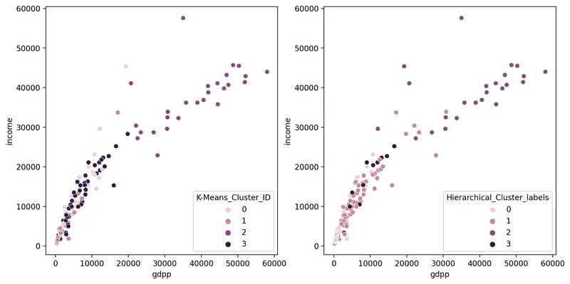

#-----------------scatter plot using the child_mort, income to observe the cluster distribution--------------------

plt.figure(figsize=(12,6),dpi=200)

plt.subplot(1,2,1)
sns.scatterplot(x='child_mort',y='income',data=country_data_outliers_removed,hue='K-Means_Cluster_ID')

plt.subplot(1,2,2)
sns.scatterplot(x='child_mort',y='income',data=country_data_outliers_removed,hue='Hierarchical_Cluster_labels')

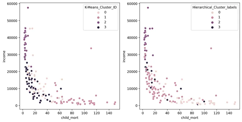
As we can observe from the above figure low income results in higher child mortality

Countries which are in direst need of aid

K_Means_countries = country_data_outliers_removed[country_data_outliers_removed['K-Means_Cluster_ID'] == 1]
Hirarchical_countries = country_data_outliers_removed[country_data_outliers_removed['Hierarchical_Cluster_labels'] == 0]
common_countries = pd.merge(K_Means_countries,Hirarchical_countries,how='inner',on=['country', 'child_mort', 'exports', 'health', 'imports', 'income',
       'inflation', 'life_expec', 'total_fer', 'gdpp', 'K-Means_Cluster_ID',
       'Hierarchical_Cluster_labels'])
common_countries.columns
common_countries_final = common_countries[['country', 'child_mort','income','gdpp']].sort_values(['child_mort','income'],ascending=[False,True])

final_countries = common_countries_final[(common_countries_final['child_mort'] > 80) &  (common_countries_final['income'] < 1200)]
final_countries = final_countries.reset_index(drop=True)
final_countries

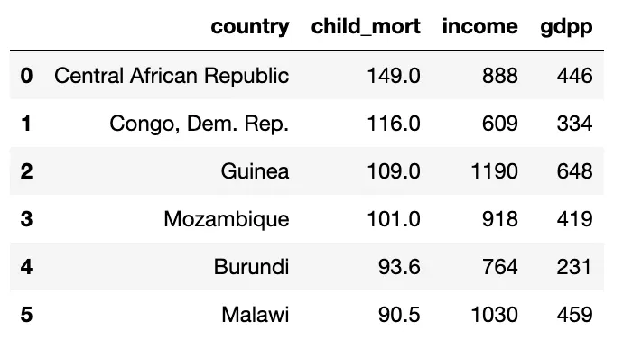
Countries that are in direst need for aid:-

1.Central African Republic

2.Congo, Dem. Rep.

3.Mozambique

4.Burundi

5.Malawi

6.Guinea

-----------------------------------------------------------------------------------------------------------------------------