Project 2
AIM
The main goal of this project is to understand the functionality of a P1 hybrid and be able to model it.
INTRODUCTION
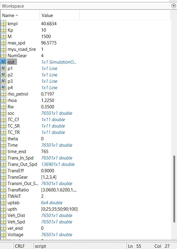
As from the name Hybrid Electric Vehicle, we know that the vehicle is powered using both IC Engine and Electric motor which helps to get great fuel efficiency. By the position of the electric motor that used to power the powertrain we can classified it into different category, so here we are going to the P1 type architecture. The P1 architecture, with the electric motor is connected directly to the crankshaft. This type of architecture helps to eliminate the starter motor and it act as a starter motor, it also acts as a generator during deceleration, and also helps to give extra power to the engine during vehicle accelerations. It can also provide high torque. Here we are going to monitor the system adopted by the Honda on there first-generation Integrated Motor Assist (IMA) technology. Data is taken from ADVISOR data base developed by NREL, USA. Data provided in the project files. They are using PMSM motor with Power of 10kW and battery capacity of 6Ah, 154V, NiMH Battery.
SIMULATION MODE
In this mode the we use forward model with dynamic stimulation. Dynamic models are also used for detailed simulation. Vehicle state variable such as velocity and acceleration are the output and force, torque, and power as the input. The simulation are more realistic and there feedback loop to meet the desired vehicle state. By using the urban drive cycle and highway drive cycle the analyse of the simulation take place.
TASK
Load the project2 file to the current folder of the Matlab
Then run the initial file “Project2_InitFile.m” in Matlab script
and then select 1 for the UDDS cycle and 2 for HWFET
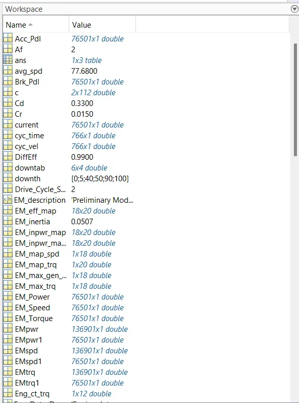
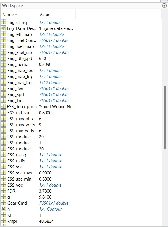
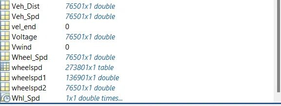
then run the program and bring all data to the workspace.
FOR UDDS
%%%%%%%%%%%%%%%%%%%%%%%%%%%%%%%%%%%%%%%%%%%%%%%%%%%%%%%%%%%%%%%%%%%%%
%% Skill-Lync -> Hybrid Drives Development
% Project  - P1 Electric Vehicle Model
% By -Aswin os

% Description:

%% Initialization File
% Initialization file for loading the variables for the Conventional vehicle simulation model

%% Vehicle Parameters
M = 1500;       % Vehicle weight [kg]
Cr = 0.015;     % Rolling resistance coefficient
Rw = 0.35;      % Rolling radius [m]
Cd = 0.33;      % Drag coefficient
Af = 2;         % Frontal area [m2]
rhoa = 1.225;   % Air density [kg/m3]
Vwind = 0;      % Wind velocity [kmph]
g = 9.81;       % Gravitational acceleration [m/s2]
theta = 0;      % Slope [deg]
myu_road_tire = 1; % Coefficient of friction between tire - road interface

%% Powertrain Parameters
FDR = 3.73;                         % Final Drive Ratio / Diff Ratio
DiffEff = 0.99;                     % Differential efficiency (assumed independent of operating conditions)

NumGear = 4;                        % Number of gears in transmission
TransGear = [1:NumGear];            % Transmission Gears
TransRatio = [3.06, 1.62, 1, 0.7];  % Corresponding Transmission ratios
TransEff = 0.90;                    % Transmission efficiency (assumed independent of operating conditions)

TC_SR = [0, .5, .6, .7, .8, .87, .92, .94, .96, .97, 1];   % Torque Converter Speed Ratio (Matlab default) -> TurbSpd/PumpSpd
TC_TR = [2.232, 1.5462, 1.4058, 1.2746, 1.1528, 1.0732, 1.0192, 1, 1, 1, 1];   % Torque Converter Torque Ratio (Matlab default) -> TurbTrq/PumpTrq
TC_Cf = 1e-4 * [.72558, .66322, .63463, .59042, .51331, .4144, .29287, .22444, .12186, .04386, 0]; % Torque Converter Capacity Factor (Matlab default) -> PumpTrq/PumpSpd^2 [Nm/rpm^2]

load Vehicle_Data/Engine_data_1_9L_Saturn_95kW
load Vehicle_Data/Trans_Shift_map
load Vehicle_Data/EM_Honda_Insight_10kW
load Vehicle_Data/ESS_NiMH6


ESS_init_soc = 0.8;
ESS_soc_max = 0.9;
ESS_soc_min = 0.6;


%% Driver Parameters
Kp = 10;                    % P gain for driver PI model
Ki = 1;                     % I gain for driver PI model
Drive_Cycle_Select = 1;     % Drive cycle selection

% Drive cycle values in m/s

if Drive_Cycle_Select == 1
    load DriveCycles/UDDS;

elseif Drive_Cycle_Select == 2
    load DriveCycles/HWFET;

elseif Drive_Cycle_Select == 3
    load DriveCycles/FTP;

elseif Drive_Cycle_Select == 4
    load DriveCycles/US06;

elseif Drive_Cycle_Select == 5
    load DriveCycles/NEDC;

elseif Drive_Cycle_Select == 6
    load DriveCycles/WLTP;

end

time_end = cyc_time(end);
vel_end = cyc_vel(end);
FOR HWFET
%%%%%%%%%%%%%%%%%%%%%%%%%%%%%%%%%%%%%%%%%%%%%%%%%%%%%%%%%%%%%%%%%%%%%
%% Skill-Lync -> Hybrid Drives Development
% Project  - P1 Electric Vehicle Model
% By -Aswin os

% Description:

%% Initialization File
% Initialization file for loading the variables for the Conventional vehicle simulation model

%% Vehicle Parameters
M = 1500;       % Vehicle weight [kg]
Cr = 0.015;     % Rolling resistance coefficient
Rw = 0.35;      % Rolling radius [m]
Cd = 0.33;      % Drag coefficient
Af = 2;         % Frontal area [m2]
rhoa = 1.225;   % Air density [kg/m3]
Vwind = 0;      % Wind velocity [kmph]
g = 9.81;       % Gravitational acceleration [m/s2]
theta = 0;      % Slope [deg]
myu_road_tire = 1; % Coefficient of friction between tire - road interface

%% Powertrain Parameters
FDR = 3.73;                         % Final Drive Ratio / Diff Ratio
DiffEff = 0.99;                     % Differential efficiency (assumed independent of operating conditions)

NumGear = 4;                        % Number of gears in transmission
TransGear = [1:NumGear];            % Transmission Gears
TransRatio = [3.06, 1.62, 1, 0.7];  % Corresponding Transmission ratios
TransEff = 0.90;                    % Transmission efficiency (assumed independent of operating conditions)

TC_SR = [0, .5, .6, .7, .8, .87, .92, .94, .96, .97, 1];   % Torque Converter Speed Ratio (Matlab default) -> TurbSpd/PumpSpd
TC_TR = [2.232, 1.5462, 1.4058, 1.2746, 1.1528, 1.0732, 1.0192, 1, 1, 1, 1];   % Torque Converter Torque Ratio (Matlab default) -> TurbTrq/PumpTrq
TC_Cf = 1e-4 * [.72558, .66322, .63463, .59042, .51331, .4144, .29287, .22444, .12186, .04386, 0]; % Torque Converter Capacity Factor (Matlab default) -> PumpTrq/PumpSpd^2 [Nm/rpm^2]

load Vehicle_Data/Engine_data_1_9L_Saturn_95kW
load Vehicle_Data/Trans_Shift_map
load Vehicle_Data/EM_Honda_Insight_10kW
load Vehicle_Data/ESS_NiMH6


ESS_init_soc = 0.8;
ESS_soc_max = 0.9;
ESS_soc_min = 0.6;


%% Driver Parameters
Kp = 10;                    % P gain for driver PI model
Ki = 1;                     % I gain for driver PI model
Drive_Cycle_Select = 2;     % Drive cycle selection

% Drive cycle values in m/s

if Drive_Cycle_Select == 1
    load DriveCycles/UDDS;

elseif Drive_Cycle_Select == 2
    load DriveCycles/HWFET;

elseif Drive_Cycle_Select == 3
    load DriveCycles/FTP;

elseif Drive_Cycle_Select == 4
    load DriveCycles/US06;

elseif Drive_Cycle_Select == 5
    load DriveCycles/NEDC;

elseif Drive_Cycle_Select == 6
    load DriveCycles/WLTP;

end

time_end = cyc_time(end);
vel_end = cyc_vel(end);
After that open the Simulink
SIMULINK MODEL
- Layout Block
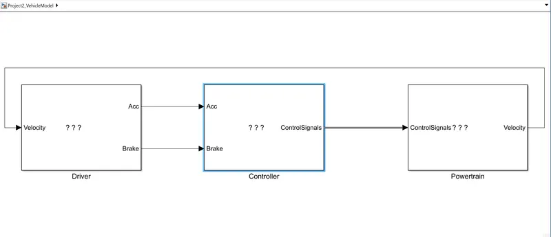
This contain three blocks, which is the Driver, Controller, Powertrains blocks.
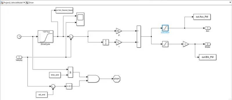
1. Driver block which is the basic P1 controller that generates the acceleration and break pedal output according to the actual speed. Drive data are used to generate the acceleration and brake output.
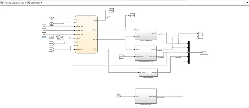
2. Controller Block is the brain of the vehicle which take the output of the driver as the input and generate desired engine torque transmission gear, motor torque and break torque. All electronic control units also include under the controller. A state flow chart is present in the controller. The state flow chart has five inputs, such as Acceleration, Brake, Engine Speed, Vehicle Speed, SOC and ClutchLockup. And have four output such as, mode, engine ON/OFF, Engine torque, Motor torque. In this chart we create four conditions as stop, start, Drive and Regenerative Braking. Corresponding state flow also represent there
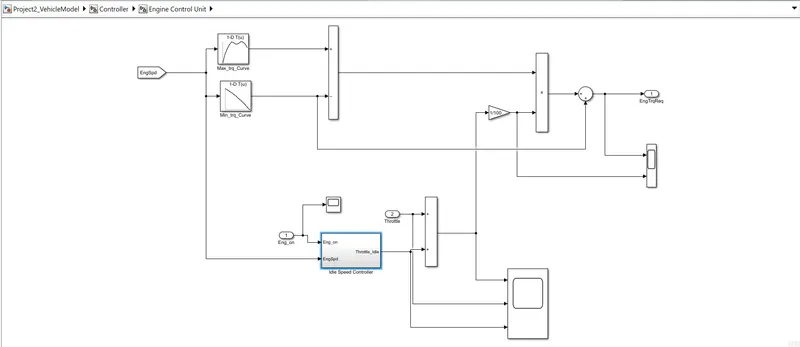
- ECU (engine control Unit)^^
We give input engine speed through a lookup table. Were input as maximum torque/map speed and ct torque/map speed.
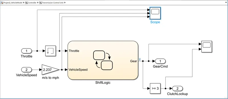
- Transmission control Unit^^
In this we create a steady flow variable state for the upshifting and downshifting of the gear
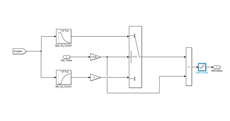
- Electric motor control unit^^
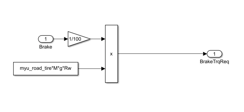
- Brake control unit^^
- Powertrain Block
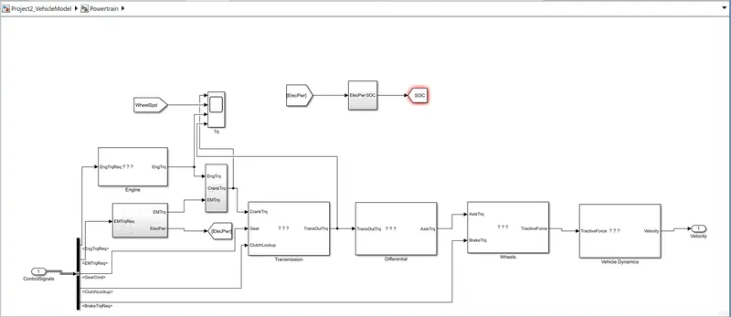
It take all the output of controller as input such as engine torque request, EM torque request, Brake torque request, gear command
The powertrain block consist of
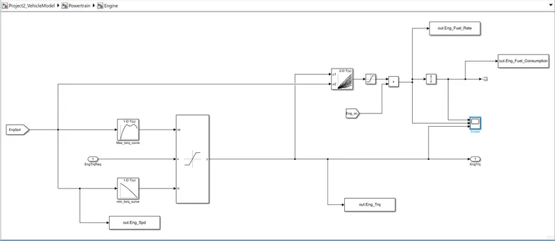
- Engine Block^^
Map based modelling is enabling in this model block, using 1D lookup table the max torque and min torque plotted and then saturated then give a out as fuel consumption and the engine torque.
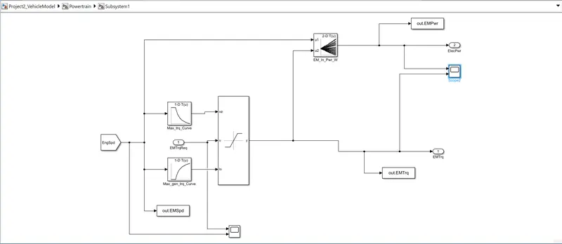
- Electric motor
- ESS
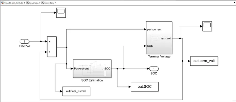
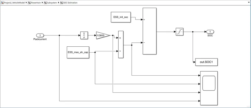
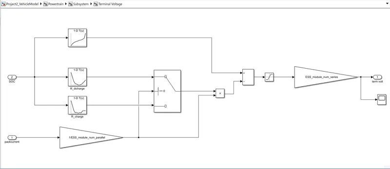
An energy storage system which stores and discharge charge when needed and has an out of SOC
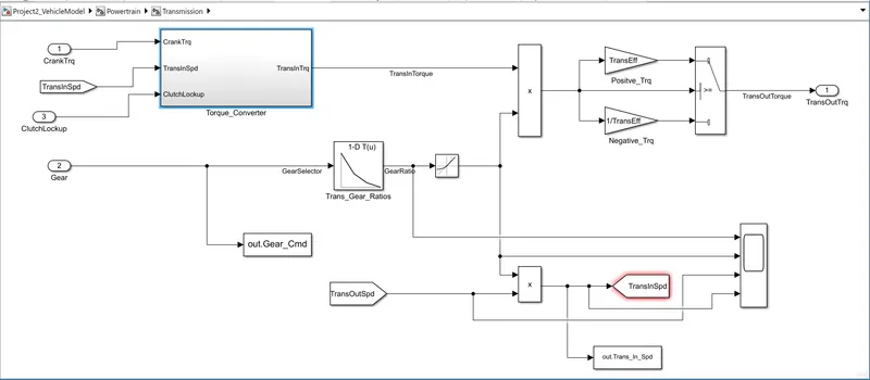
- Transmission Unit
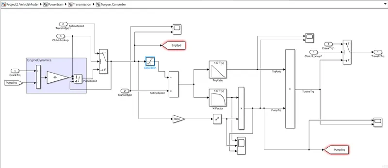
Torque Convertor
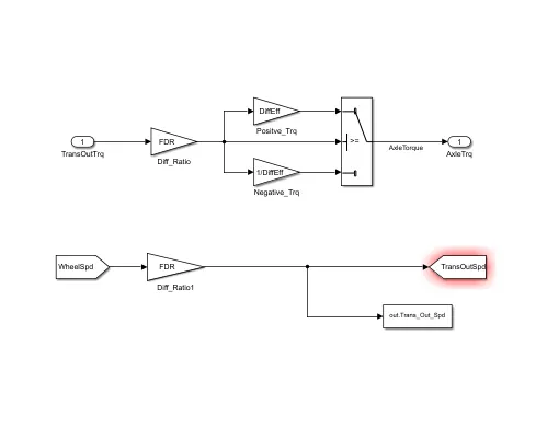
- Differential unit
- Wheels
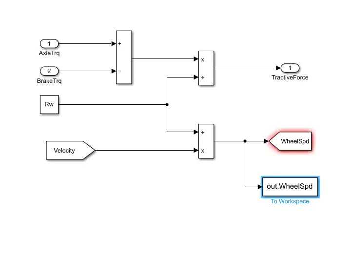
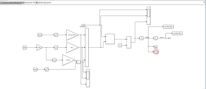
Vehicle Dynamics
POST PROCESSING
%%%%%%%%%%%%%%%%%%%%%%%%%%%%%%%%%%%%%%%%%%%%%%%%%%%%%%%%%%%%%%%%%%%%%
%% Skill-Lync -> Hybrid Drives Development
% Project  - P1 Electric Vehicle Model
% By -Aswin os
% Description:
% The following file is to used with the Initialization file and Simulink
% results for post-processing of the data.
% The file is incomplete, has some examples of how the data is imported
% into a readable format, data analysis and plotting examples.
% Based on the project task, use commands in a similar format as given
% below, to analyse the data and generate required plots.
% You can change variable names if desired

%% Post-Processing File
%  File for post-processing the Conventional vehicle simulation model data

%% Renaming variables
Time = out.tout;
Acc_Pdl = out.Acc_Pdl;          % Accelerator pedal [%]
Brk_Pdl = out.Brk_Pdl;         % Brake pedal [%]
Gear_Cmd = out.Gear_Cmd;        % Transmission gear
Trans_In_Spd = out.Trans_In_Spd*30/pi;  % Transmission input speed [rpm]
Transm_Out_Spd =Trans_Out_Spd*30/pi;% Transmission output speed [rpm]
Eng_Trq = out.Eng_Trq;          % Engine brake torque [Nm]
Eng_Spd = out.Eng_Spd*30/pi;    % Engine speed [rpm]
Eng_Fuel_Consump = out.Eng_Fuel_Consumption;    % Engine fuel consumption [g]
Veh_Dist = out.Veh_Dist/1000;   % Distance traveled by vehicle [km]
Veh_Spd = out.Veh_Spd*18/5;     % Vehicle speed [kmph]
Wheel_Spd = wheelspd1;         %Wheel speed in kmpl
Eng_Fuel_rate= out.Eng_Fuel_Rate; %engine fuel rate[%]
EM_Speed= EMspd*18/5;       %electric motor speed
EM_Power= EMpwr;             %electric motor power
EM_Torque= EMtrq;            %electric motor torque
soc= out.SOC;                 %Source of charge
Voltage = out.term_volt;      %Terminal voltage of battery
current=out.Pack_Current;      %Pack current of battery

%% Data Analysis
Eng_Pwr = Eng_Spd.*pi/30.*Eng_Trq/1000;   % Engine brake power [kW]
rho_petrol = 0.7197;                    % Density of petrol [kg/L]
kmpl = Veh_Dist(end)/(Eng_Fuel_Consump(end)/1000/rho_petrol);    % Fuel economy [kmpl]


%% Plotting Transmission input trransmission output and wheel speed
figure(1)
hold on
grid on
plot(Time, Trans_In_Spd, 'linewidth', 1, 'Color', 'black')
plot(Time, Transm_Out_Spd, 'linewidth', 1, 'Color', 'black')
plot(Time, Wheel_Spd', 'linewidth', 1, 'Color', 'blue')
xlabel('time in s')
ylabel('speed in rpm')
xlim([0,Time(end)])
ylim([0, 6000])
legend('Transmission input','transmission output','Wheelspeed')

%% Plotting vehicle characteristics time trace
figure(2)
subplot(3,1,1)
hold on
grid on
plot(Time, Acc_Pdl, 'linewidth', 1, 'Color', 'black');
plot(Time, Brk_Pdl, 'linewidth', 1, 'Color', 'red');
ylabel('Pedal [%]')
xlim([0, Time(end)]);
legend('Accel','Brake');
subplot(3,1,2)
hold on
grid on
plot(Time, Trans_In_Spd, 'linewidth', 1, 'Color', 'black');
plot(Time, Trans_Out_Spd, 'linewidth', 1, 'Color', 'red');
ylabel('Speed [rpm]')
xlim([0, Time(end)]);
ylim([0, 6000]);
legend('Trans Input','Trans Output');
subplot(3,1,3)
hold on
grid on
plot(Time, Gear_Cmd,'linewidth', 1, 'Color', 'black');
xlim([0, Time(end)]);
xlabel('Time [s]');
ylabel('Gear');
%% plotting engine torque, engine power, fuel rate and fuel consumption
figure(3)
subplot(4,1,1)
hold on
grid on
plot(Time, Eng_Trq, 'linewidth', 1, 'Color', 'black');
ylabel('Torquein Nm');
xlim([0,Time(end)]);
subplot(4,1,2)
hold on
grid on
plot(Time, Eng_Pwr, 'linewidth', 1, 'Color', 'black');
ylabel('Power in kW');
xlim([0,Time(end)]);
subplot(4,1,3)
hold on
grid on
plot(Time, Eng_Fuel_Consump, 'linewidth', 1, 'Color', 'black');
xlabel('time')
ylabel('Engine fuel consumption');
xlim([0,Time(end)]);
subplot(4,1,4)
hold on
grid on
plot(Time, Eng_Fuel_rate, 'linewidth', 1, 'Color', 'black');
xlabel('time')
ylabel('Engine fuel rate in %');
xlim([0,Time(end)]);
%% Plotting engine operating points on engine fuel map
figure('Name','Engine Operating Points');
hold on
grid on
title('Engine Operating Points','fontsize',12);
p1=plot(Eng_map_spd*30/pi,Eng_max_trq,'linewidth',2,'color','r');
p2=line([Eng_map_spd(end)*30/pi Eng_map_spd(end)*30/pi],[0 Eng_max_trq(end)]);
set(p2,'linewidth',1,'linestyle','--','color','k');
p3=line([Eng_map_spd(1)*30/pi Eng_map_spd(1)*30/pi],[0 Eng_max_trq(1)]);
set(p3,'linewidth',1,'linestyle','--','color','k');
[c,h] = contour(Eng_map_spd'*30/pi,Eng_map_trq,Eng_fuel_map');
clabel(c,h);
xlabel('Engine Speed [rpm]');
ylabel('Engine Torque [Nm]');
title('Engine Fuel Consumption Map [g/s]');
p4 = plot(Eng_Spd,Eng_Trq,'.','color','k');
legend([p1 p4],{'Max Curve','Operating Points'});
axis([Eng_map_spd(1)*30/pi Eng_map_spd(end)*30/pi 0 Eng_map_trq(end)]);

%% Plotting of Gear command of vehicle at desired speed and distance
figure(6)
hold on
grid on
subplot(2,1,1)
plot(Veh_Spd, Gear_Cmd,'linewidth', 1, 'Color', 'black');
xlabel('Speed in kmph')
ylabel('Gear')
title('Gear command according to speed ')
subplot(2,1,2)
plot(Veh_Dist, Gear_Cmd,'linewidth', 1, 'Color', 'black');
xlabel('distancee in km');
ylabel('Gear');
title('Gear command according to Distance ');


%% plottting drive cycle
figure(5)
hold on
grid on
plot(cyc_time, cyc_vel,'LineWidth',1,'Color','black');
xlabel('time in s');
ylabel('velocity in mph');
title('drive cycle');
%% plotiing the Charge pack,soc,and terminal voltage with time trace
figure(7)
subplot(3,1,1)
hold on
grid on
plot(Time, current, 'linewidth', 1, 'Color', 'black');
xlabel('time');
ylabel('Pack Current');
xlim([0, Time(end)]);
legend('Pack current');

subplot(3,1,2)
hold on
grid on
plot(Time, soc, 'linewidth', 1, 'Color', 'red');
xlabel('time');
ylabel('Charging');
xlim([0, Time(end)]);
legend('State of charge');

subplot(3,1,3)
hold on
grid on
plot(Time, Voltage,'linewidth', 1, 'Color', 'blue');
xlim([0, Time(end)]);
xlabel('Time [s]');
ylabel('T Voltage in v');
legend('terminal voltage');
%% plotting motor spped torque and input power
figure(8)
subplot(3,1,1)
hold on
grid on
plot(Time, EM_Power, 'linewidth', 1, 'Color', 'black');
xlabel('time');
ylabel('Motor power');
xlim([0, Time(end)]);
legend('EM Power');

subplot(3,1,2)
hold on
grid on
plot(Time,EM_Speed, 'linewidth', 1, 'Color', 'red');
xlabel('time');
ylabel('Motor speed');
xlim([0, Time(end)]);
legend('EM Speed');

subplot(3,1,3)
hold on
grid on
plot(Time, EM_Torque,'linewidth', 1, 'Color', 'blue');
xlim([0, Time(end)]);
xlabel('Time [s]');
ylabel('motor torque');
legend('EM Torque');

%% Plotting EM operating points on Inputpower map
figure('Name','EM Operating Points');
hold on
grid on
title('EM Operating Points','fontsize',12);
p1=plot(EM_map_spd*30/pi,EM_max_trq,'linewidth',2,'color','r');
p2=line([EM_map_spd(end)*30/pi EM_map_spd(end)*30/pi],[0 EM_max_trq(end)]);
set(p2,'linewidth',1,'linestyle','--','color','k');
p3=line([EM_map_spd(1)*30/pi EM_map_spd(1)*30/pi],[0 EM_max_trq(1)]);
set(p3,'linewidth',1,'linestyle','--','color','k');
[c,h] = contour(EM_map_spd'*30/pi,EM_map_trq,EM_inpwr_map');
clabel(c,h);
xlabel('EM Speed [rpm]');
ylabel('EM Torque [Nm]');
title('EM input power  Map [g/s]');
p4 = plot(Eng_Spd,Eng_Trq,'.','color','k');
legend([p1 p4],{'Max Curve','Operating Points'});
axis([EM_map_spd(1)*30/pi EM_map_spd(end)*30/pi 0 EM_map_trq(end)]);
%% test result
avg_spd=sum(Veh_Spd)/length(Veh_Spd);
max_spd=maxk(Veh_Spd,1);
table(avg_spd,max_spd,kmpl,'VariableNames',{'Average speed[kmpl]','Maximum speed[kmpl]','Fuel economy[kmpl]'})
TEST RESULTS
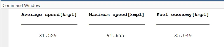
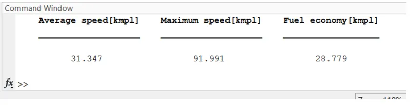
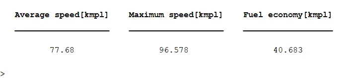
a. Tabulate the fuel economy numbers (kmpl) for UDDS and HWFET cycle. Compare these numbers with the baseline numbers for conventional vehicle model from Project 1.
UDDS CYCLE FUEL ECONOMY FOR HEV
UDDS CYCLE FUEL ECONOMY FOR CONVENTION VEHICLE IN PROJECT 1
HWFET CYCLE FUEL ECONOMY FOR HEV
HWFET CYCLE FUEL ECONOMY FOR CONVENTION VEHICLE IN PROJECT 1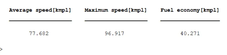
From the fuel consumption in KMPL it is clear that in city ride an HEV can provide a 10% extra fuel efficiency than the conventional IC engine vehicle, But in highway ride its giviing almost same fuel economy. While compairing between the USSD And HWFETCycle the HWFET have the highest fuel economy.
Plot the time trace for engine, transmission input, transmission output and wheel speed on one plot.
USSD
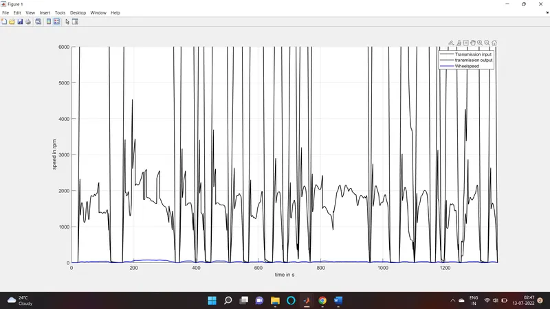
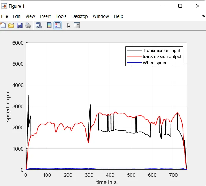
In this we can see that the USSD showing more fluctuations on that the Highway cycle it beacuse of the rapid start stop and breaking .
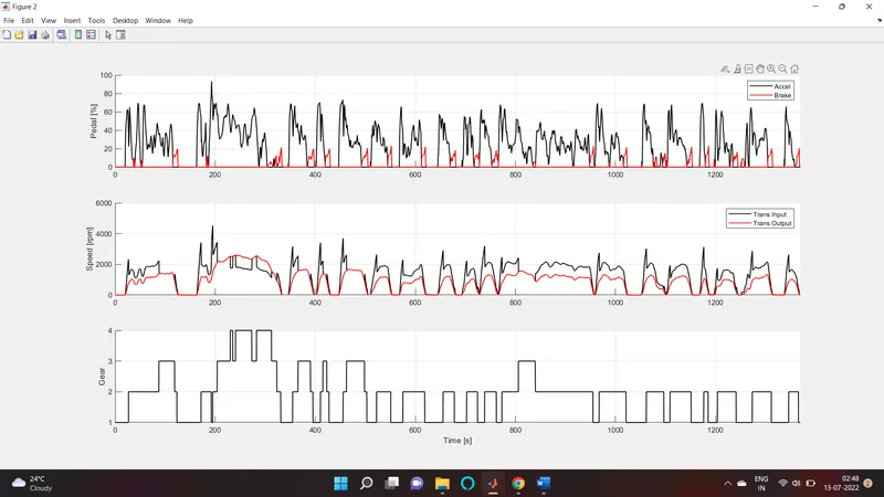
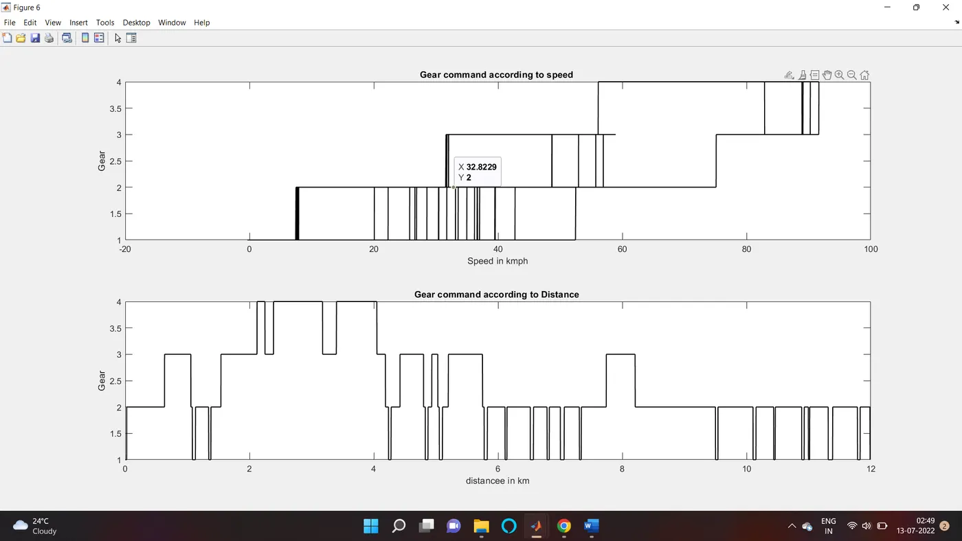
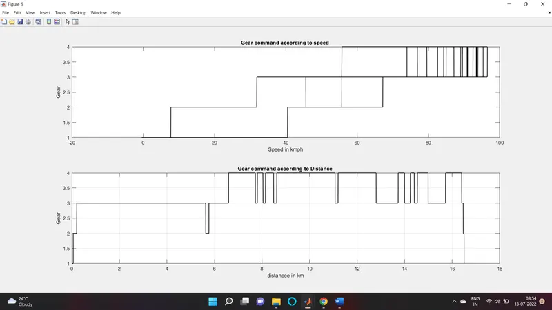
Plot accelerator and brake pedal, gear command, vehicle desired and actual speed, vehicle distance using subplots.
HWFET
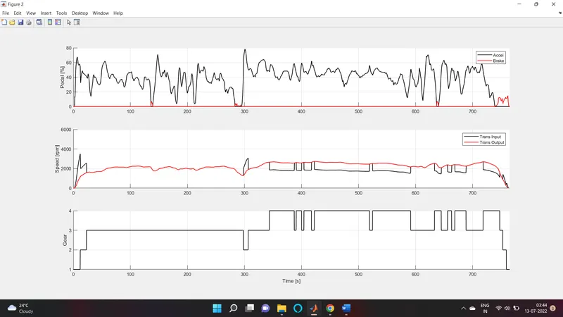
In UDDS cycle mostly runs on 1st and 2nd gears and the 3rd and 4th gears are rarely useas it does not achieve high speed inn that traffic. In The HWFET cycle the vehicle mostly runn in 3rd and 4th gears as it will moving at high speeds.
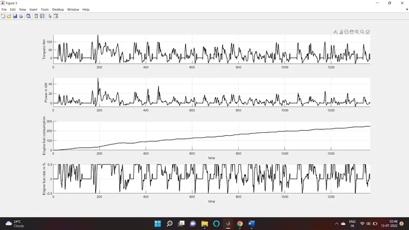
Plot engine torque, engine power, fuel rate and fuel consumption using subplots.
USSD
HWFET
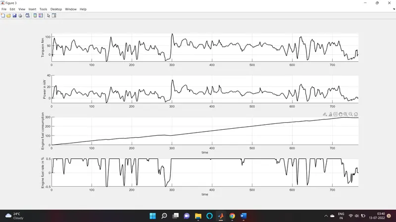
Vehicle cosumed more power in UDDS drive ccycle bacause in urban area the vehicle require many starts and stops so it required more power compred to HWFET.
In order to overcome the static friction in USSD Cycle engine need more power.
the fuel rate is high in HWFET beacuse of the continous movement.
Fuel economy is high for HWFET because USSD have rapid start stop which consume more fuel
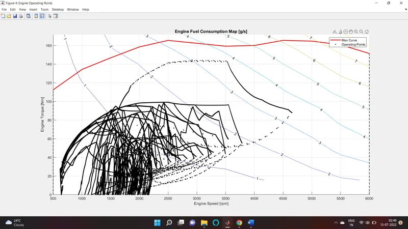
Plot the engine operating points on the engine fuel map.
USSD
Plot accelerator and brake pedal, gear command, vehicle desired and actual speed, vehicle distance using subplots
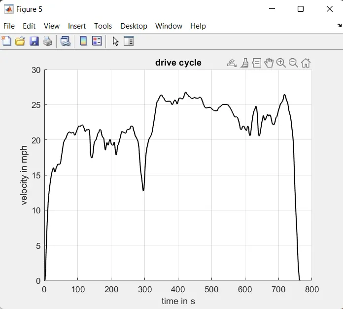
HWFET
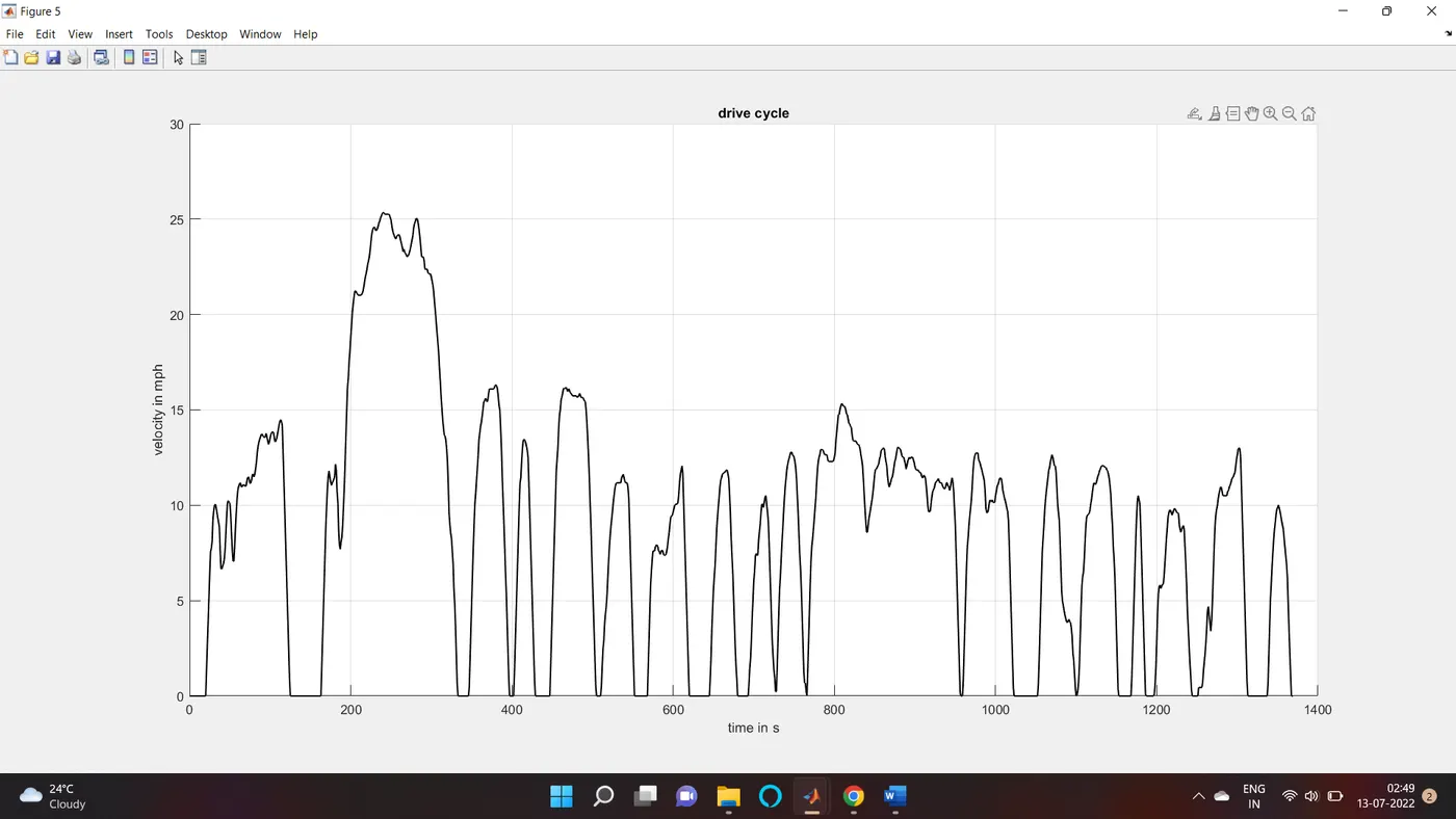
Drive Cycle
USSD
HWFET
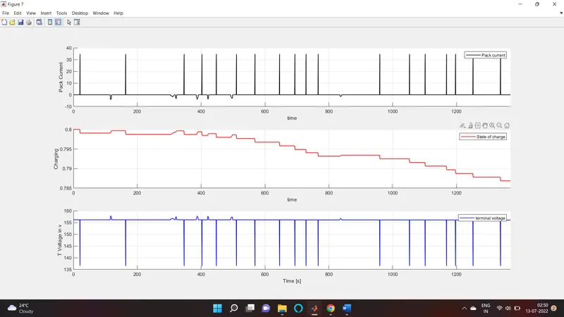
Plot pack voltage, current and SoC using subplots
HWFET
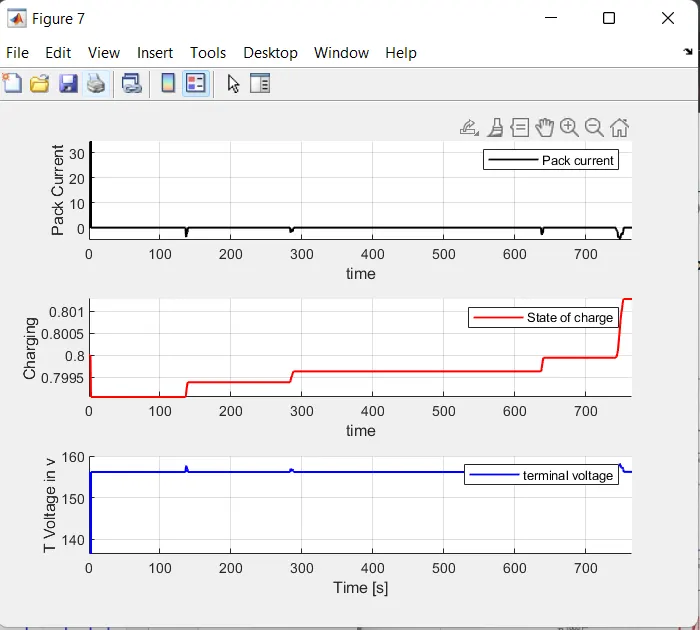 The pack current and terminal voltage will have more flectuation when compare to the HWFET cycle with USSD. it is because of the radip stop and start in city ride where the motor need to work more.
SOC decreases in USSD with time and increases with HWFET
Plot motor speed, torque, motor input power using subplots.
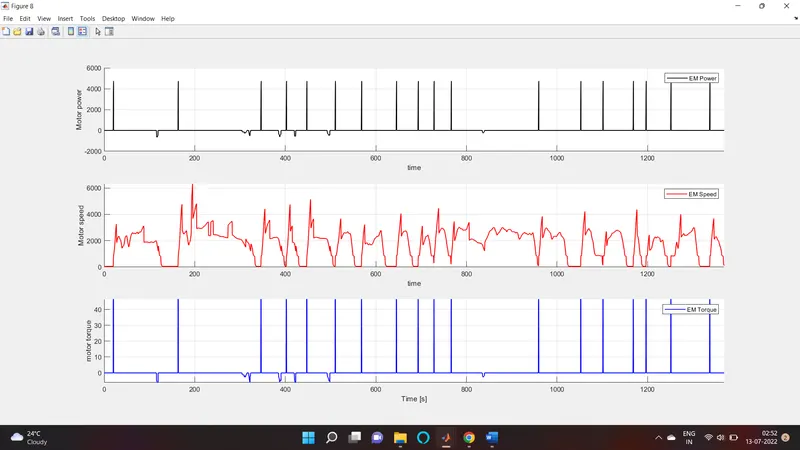
HWFET
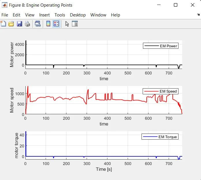
we can see that the power and torque are very high in HWFET at initial condition and they are almost zero after some times but in USSD its has continuos flectuation due to the frequent breaking in ussd cycle.
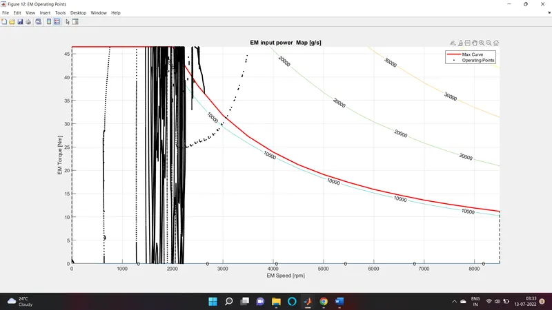
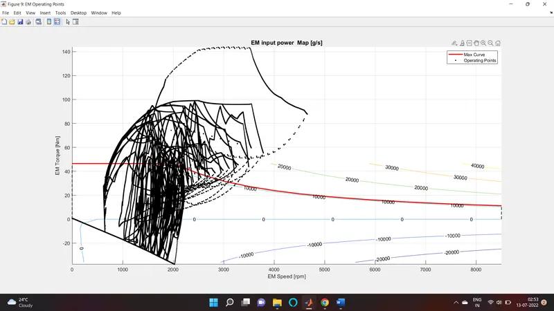
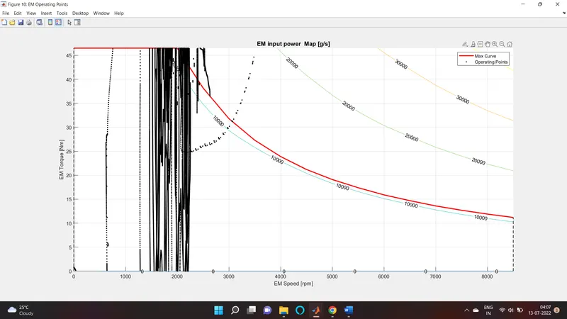
Plot the motor operating points on the motor input power map, with the motor max motoring and generating torque curves.
CONCLUSION
By using the USSD and HWFET drive cycle we able to perfome various charecteristics and condition to a vehicle model and able to understand the behaviour thus we plotted the following graphs and task
a. Tabulate the fuel economy numbers (kmpl) for UDDS and HWFET cycle. Compare these numbers with the baseline numbers for conventional vehicle model from Project 1.
b. Plot the time trace for engine, transmission input, transmission output and wheel speed on one plot.
c. Plot engine torque, engine power, fuel rate and fuel consumption using subplots.
d. Plot accelerator and brake pedal, gear command, vehicle desired and actual speed, vehicle distance using subplots.
e. Plot the engine operating points on the engine fuel map.
f. Plot motor speed, torque, motor input power using subplots.
g. Plot pack voltage, current and SoC using subplots.
h. Plot the motor operating points on the motor input power map, with the motor max motoring and generating torque curves.
i. Write down appropriate brief comments on each of these plots, describing the vehicle behavior throughout the drive cycle.
j. Generate the plots for both drive cycles
REFERANCE
Google, skill lync officials,etc
Thank you...