Project 2 - Rankine cycle Simulator
REPORT
Rankine Stimulator
Rankine cycle consist of four processes as follows.
Process 1-2: Reversible adiabatic expansion in the turbine (or steam engine).
Process 2-3: Constant-pressure transfer of heat in the condenser.
Process 3-4: Reversible adiabatic pumping in the feed pump.
Process 4-1: Constant-pressure transfer of heat in boiler.
Applying steady flow energy equation (S.F.E.E) to boiler ,turbine , condenser and pump:
- For Boiler as the control volume, we get
hf4 +Q4=h1
Q1=h1-hf4
- For turbine as the control volume, we get
h1=wt+h2 , where wt= turbine work
wt=h1-h2
- For condenser, we get
h2=Q2+hf3
Q2=h2-hf3
- For the feed pump, we get
hf3+wp=hf4
wp=hf4-hf3
Efficiency of the Rankine cycle is given by,
Effi.mu=w/Qnet1=wp/Q1
Main code explanation
Before we writing this program ,we are using XSteam.m which is basically a steam table
close all
clear all
clc
- Clearing workspace, command window ad close all plots.
%Print process Desscription
fprintf('1-2 Isobaric heat Transfer\n')
fprintf('2-3 Isentropic Expansion\n')
fprintf('3-4 Isobaric heat Rejection\n')
fprintf('4-1 Isentropoic compression \n')
- Print description of all process in the command window.
%step-1:Enter Input
p1=input('Enter the preassure at the turbine inlet(in bar): ');
T1=input('Enter the Trmperature at the turbine inlet (in degree Celcius): ');
p2=input('Enter the pressure at the condenser(in bar): ');
- Taking all input argument.
%step-2 calculate each state point values.
% State Points -1
h1=XSteam('h_pt',p1,T1);
s1=XSteam('s_pt',p1,T1);
%Step-3: state point 2
s2=s1;
sf2=XSteam('sL_p',p2);
sg2=XSteam('sV_p',p2);
hf2=XSteam('hL_p',p2);
hg2=XSteam('hV_p',p2);
T2=XSteam('Tsat_p',p2);
x2=(s2-sf2)/(sg2-sf2);
h2=hf2+(x2*(hg2-hf2));
%step 4:state point 3
p3=p2;
T3=XSteam('Tsat_p',p3);
s3=XSteam('sL_p',p3);
h3=XSteam('hL_p',p3);
%step-5 : state point 4
p4=p1;
s4=s3;
Cp4=XSteam('Cp_ps',p4,s4);
Cv4=XSteam('Cv_ps',p4,s4);
%calculating gamma
gamma=Cp4/Cv4;
r=(gamma-1)/gamma;
T4=T3*(p4/p3).^r;
h4=XSteam('h_ps',p4,s4);
%step 6 Calculate other output values
%turbine work
wt=h1-h2;
%pump work
wp=h4-h3;
w_net=wt-wp; %network unit in kg/kg
Qi=h1-h4; %heat supplied
Qo=h2-h3; %heat rejected
N_per=(w_net/Qi).*100; %efficiency
SSC= 3600/(wt-wp) ; %steam rate per second
Bwr=Qi/Qo;
- Calculation of cp values at p1 &p2 for saturated liquid and vapour.
- Calculation of saturation temperature at p1 and p2.
- Calculation of saturation property, process property of different stages.
- Calculation of work done, heat, SC and efficiency.
%step 7: statepoint 5 and 6 which help in plotting
T5=XSteam('Tsat_p',p1);
T6=T5;
s5=XSteam('sL_p',p1);
s6=XSteam('sV_p',p1);
h5=XSteam('hL_p',p1);
h6=XSteam('hV_p',p1);
%plotting the required graph
%T-S graph
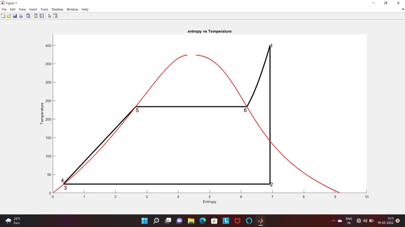
figure(1)
T_r1=linspace(T5,T1,500);
for i=1:length(T_r1)
s(i)=XSteam('s_pt',p1,T_r1(i));
end
hold on
plot([s1 s2 s3 s4 s5 s6 s],[T1 T2 T3 T4 T5 T6 T_r1],'LineWidth',3,'Color','k')
axis([0 10 0 430])
text(s1,T1,'1','FontSize',15)
text(s2,T2,'2','FontSize',15)
text(s3,T3,'3','FontSize',15,'VerticalAlignment','top')
text(s4,T4,'4','FontSize',15,'VerticalAlignment','bottom','HorizontalAlignment','right')
text(s5,T5,'5','FontSize',15,'VerticalAlignment','top')
text(s6,T6,'6','FontSize',15,'VerticalAlignment','top','HorizontalAlignment','right')
T_r2=linspace(0,T1,500);
for j = 1: length(T_r2)
sl(j)=XSteam('sL_T',T_r2(j));
sv(j)=XSteam('sv_T',T_r2(j));
hl(j)=XSteam('hL_T',T_r2(j));
hv(j)=XSteam('hv_T',T_r2(j));
end
plot(sl,T_r2,'LineWidth',1.5,'Color','r')
plot(sv,T_r2,'LineWidth',1.5,'Color','r')
xlabel('Entropy')
ylabel('Temperature')
title('entropy vs Temperature')
%H-S Graph
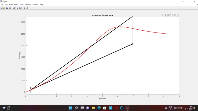
figure(2)
hold on
plot([s1 s2 s3 s4 s1],[h1 h2 h3 h4 h1],'LineWidth',3,'Color','k')
axis([0 10 -100 1000])
text(s1,h1,'1','FontSize',15)
text(s2,h2,'2','FontSize',15)
text(s3,h3,'3','FontSize',15,'VerticalAlignment','top','HorizontalAlignment','right')
text(s4,h4,'4','FontSize',15,'VerticalAlignment','bottom','HorizontalAlignment','right')
plot(sv,hv,'LineWidth',1.5,'Color','r')
plot(sl,hl,'LineWidth',1.5,'Color','r')
xlabel('Entropy')
ylabel('enthalpy')
title('entropy vs Temperature')
- Calculation and plotting of saturation liquid and vapour lines.
- Plotting T-s plot
- Plotting h-s plot
%Displaying the results
fprintf('\n______RESULTS_______\n')
fprintf('\n At State Point 1 : \n')
fprintf('P1 is : %f Bar \n',p1)
fprintf('T1 is : %f Deg Celcius \n',T1)
fprintf('H1 is : %f kJ/kg \n',h1)
fprintf('S1 is : %f kJ/kgK\n',s1)
fprintf('\n At State Point 2 : \n')
fprintf('P2 is : %f Bar \n',p1)
fprintf('T2 is : %f Deg Celcius \n',T2)
fprintf('H2 is : %f kJ/kg \n',h2)
fprintf('S2 is : %f kJ/kgK\n',s2)
fprintf('X2 is : %f \n',x2)
fprintf('\n At State Point 3 : \n')
fprintf('P3 is : %f Bar \n',p3)
fprintf('T3 is : %f Deg Celcius \n',T3)
fprintf('H3 is : %f kJ/kg \n',h3)
fprintf('S3 is : %f kJ/kgK\n',s3)
fprintf('\n At State Point 4 : \n')
fprintf('P4 is : %f Bar \n',p4)
fprintf('T4 is : %f Deg Celcius \n',T4)
fprintf('H4 is : %f kJ/kg \n',h4)
fprintf('S4 is : %f kJ/kgK\n',s4)
fprintf('wt : %f kJ/kg\n',wt)
fprintf('wp : %f kJ/kg\n',wp)
fprintf('wnet : %f kJ/kg \n',w_net)
fprintf('Ntherm : %f percent\n',N_per)
fprintf('SSC is : %f kg/kwh\n',SSC)
fprintf('BWR is : %f \n',Bwr)
- Displaying all output
MAIN CODE
close all
clear all
clc

%Print process Desscription
fprintf('1-2 Isobaric heat Transfer\n')
fprintf('2-3 Isentropic Expansion\n')
fprintf('3-4 Isobaric heat Rejection\n')
fprintf('4-1 Isentropoic compression \n')

%step-1:Enter Input
p1=input('Enter the preassure at the turbine inlet(in bar): ');
T1=input('Enter the Trmperature at the turbine inlet (in degree Celcius): ');
p2=input('Enter the pressure at the condenser(in bar): ');

%step-2 calculate each state point values.
% State Points -1
h1=XSteam('h_pt',p1,T1);
s1=XSteam('s_pt',p1,T1);

%Step-3: state point 2
s2=s1;
sf2=XSteam('sL_p',p2);
sg2=XSteam('sV_p',p2);
hf2=XSteam('hL_p',p2);
hg2=XSteam('hV_p',p2);

T2=XSteam('Tsat_p',p2);
x2=(s2-sf2)/(sg2-sf2);
h2=hf2+(x2*(hg2-hf2));
%step 4:state point 3
p3=p2;
T3=XSteam('Tsat_p',p3);
s3=XSteam('sL_p',p3);
h3=XSteam('hL_p',p3);


%step-5 : state point 4
p4=p1;
s4=s3;
Cp4=XSteam('Cp_ps',p4,s4);
Cv4=XSteam('Cv_ps',p4,s4);
%calculating gamma
gamma=Cp4/Cv4;
r=(gamma-1)/gamma;
T4=T3*(p4/p3).^r;
h4=XSteam('h_ps',p4,s4);
%step 6 Calculate other output values
%turbine work
wt=h1-h2;
%pump work
wp=h4-h3;

w_net=wt-wp;  %network unit in kg/kg
Qi=h1-h4; %heat supplied
Qo=h2-h3; %heat rejected

N_per=(w_net/Qi).*100; %efficiency
SSC= 3600/(wt-wp) ; %steam rate per second
Bwr=Qi/Qo;

%step 7: statepoint 5 and 6 which help in plotting
T5=XSteam('Tsat_p',p1);
T6=T5;
s5=XSteam('sL_p',p1);
s6=XSteam('sV_p',p1);
h5=XSteam('hL_p',p1);
h6=XSteam('hV_p',p1);

%plotting the required graph

%T-S graph
figure(1)
T_r1=linspace(T5,T1,500);
for i=1:length(T_r1)
    s(i)=XSteam('s_pt',p1,T_r1(i));
end
hold on
plot([s1 s2 s3 s4 s5 s6 s],[T1 T2 T3 T4 T5 T6 T_r1],'LineWidth',3,'Color','k')
axis([0 10 0 430])
text(s1,T1,'1','FontSize',15)
text(s2,T2,'2','FontSize',15)
text(s3,T3,'3','FontSize',15,'VerticalAlignment','top')
text(s4,T4,'4','FontSize',15,'VerticalAlignment','bottom','HorizontalAlignment','right')
text(s5,T5,'5','FontSize',15,'VerticalAlignment','top')
text(s6,T6,'6','FontSize',15,'VerticalAlignment','top','HorizontalAlignment','right')

T_r2=linspace(0,T1,500);
for j = 1: length(T_r2)
    sl(j)=XSteam('sL_T',T_r2(j));
    sv(j)=XSteam('sv_T',T_r2(j));
    hl(j)=XSteam('hL_T',T_r2(j));
    hv(j)=XSteam('hv_T',T_r2(j));
end
plot(sl,T_r2,'LineWidth',1.5,'Color','r')
plot(sv,T_r2,'LineWidth',1.5,'Color','r')
xlabel('Entropy')
ylabel('Temperature')
title('entropy vs Temperature')

%H-S Graph
figure(2)
hold on
plot([s1 s2 s3 s4 s1],[h1 h2 h3 h4 h1],'LineWidth',3,'Color','k')
axis([0 10 -100 1000])
text(s1,h1,'1','FontSize',15)
text(s2,h2,'2','FontSize',15)
text(s3,h3,'3','FontSize',15,'VerticalAlignment','top','HorizontalAlignment','right')
text(s4,h4,'4','FontSize',15,'VerticalAlignment','bottom','HorizontalAlignment','right')


plot(sv,hv,'LineWidth',1.5,'Color','r')
plot(sl,hl,'LineWidth',1.5,'Color','r')
xlabel('Entropy')
ylabel('enthalpy')
title('enthalpy vs Temperature')

%Displaying the results
fprintf('\n______RESULTS_______\n')
fprintf('\n At State Point 1 : \n')
fprintf('P1 is : %f Bar \n',p1)
fprintf('T1 is : %f Deg Celcius \n',T1)
fprintf('H1 is : %f kJ/kg \n',h1)
fprintf('S1 is : %f kJ/kgK\n',s1)

fprintf('\n At State Point 2 : \n')
fprintf('P2 is : %f Bar \n',p1)
fprintf('T2 is : %f Deg Celcius \n',T2)
fprintf('H2 is : %f kJ/kg \n',h2)
fprintf('S2 is : %f kJ/kgK\n',s2)
fprintf('X2 is : %f \n',x2)

fprintf('\n At State Point 3 : \n')
fprintf('P3 is : %f Bar \n',p3)
fprintf('T3 is : %f Deg Celcius \n',T3)
fprintf('H3 is : %f kJ/kg \n',h3)
fprintf('S3 is : %f kJ/kgK\n',s3)

fprintf('\n At State Point 4 : \n')
fprintf('P4 is : %f Bar \n',p4)
fprintf('T4 is : %f Deg Celcius \n',T4)
fprintf('H4 is : %f kJ/kg \n',h4)
fprintf('S4 is : %f kJ/kgK\n',s4)


fprintf('wt : %f kJ/kg\n',wt)
fprintf('wp : %f  kJ/kg\n',wp)
fprintf('wnet : %f kJ/kg \n',w_net)
fprintf('Ntherm : %f percent\n',N_per)
fprintf('SSC is : %f kg/kwh\n',SSC)
fprintf('BWR is : %f \n',Bwr)
RESULT
input inlet tuerbine temperature of 400degree celcius
inlet pressure of turbine of 30bar
presure at condenser is 0.05bar
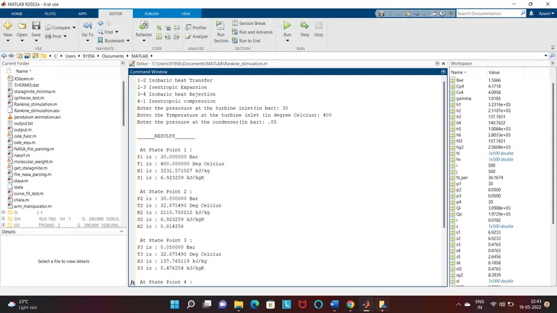
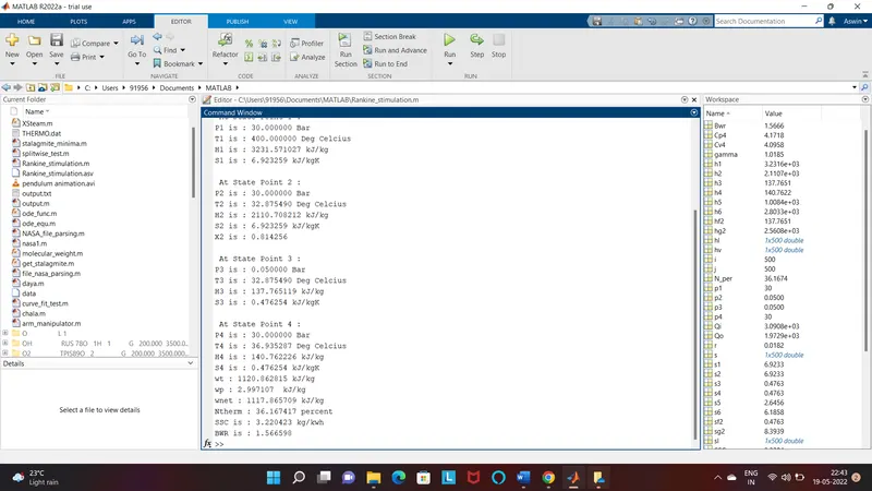
Graph of Entropy vs Temperature
Graph of Enthalpy vs Temperature