Project 2

# Project No. 2

As discussed in Lecture 11, Project 2 deals with the development of a forward energy-based fuel consumption model of a P1 hybrid vehicle. This model is based on the conventional vehicle model from Project 1.

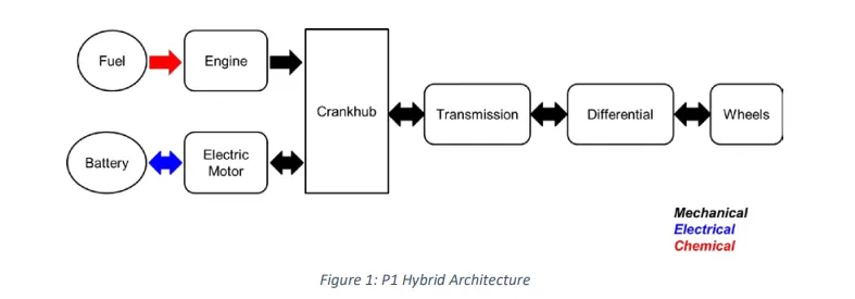
The main goal of this project is to understand the functionality of a P1 hybrid and be able to model it.

Honda Insight motor and battery are considered for this project. Data is taken from ADVISOR data base developed by NREL, USA. Data provided in the project files.

“Project2_InitFile.m” is a Matlab script used to load all the variables required for running the Simulink model and for post-processing. The drive cycle selection is also done here. Before running the Simulink vehicle model, run this initialization script.

Task:

The task of this project is to quantify the improvement in fuel economy numbers for the hybrid vehicle (kmpl), compared to the conventional vehicle, on the urban cycle (UDDS) and highway cycle (HWFET). Also, to analyze and understand the vehicle operating points in terms of engine and motor speed, torque, transmission speeds, pedal positions, gear, distance traveled, battery voltage, current, SoC etc.

To do that, the following steps need to be followed:

1) Load the Project2 folder as the Current Folder in Matlab.
2) Run the “Project2_InitFile.m” Matlab script.
3) Copy the Conventional vehicle Simulink model created for Project 1 in this folder. Figure 1: P1 Hybrid ArchitectureHybrid Drives Development
4) Modify this model into a hybrid vehicle model. The lecture presentations can be used as reference. Battery and Supervisory controller models developed in the assignments can be reused.
5) Add additional ‘To Workspace’ blocks for transferring the desired Simulink vehicle data into the Matlab workspace.
6) Simulate the hybrid model on the desired drive cycles.
7) Write a project report that contains the following:
a. Tabulate the fuel economy numbers (kmpl) for UDDS and HWFET cycle. Compare these numbers with the baseline numbers for conventional vehicle model from Project 1.
b. Plot the time trace for engine, transmission input, transmission output and wheel speed on one plot.
c. Plot engine torque, engine power, fuel rate and fuel consumption using subplots.
d. Plot accelerator and brake pedal, gear command, vehicle desired and actual speed, vehicle distance using subplots.
e. Plot the engine operating points on the engine fuel map.
f. Plot motor speed, torque, motor input power using subplots.
g. Plot pack voltage, current and SoC using subplots.
h. Plot the motor operating points on the motor input power map, with the motor max motoring and generating torque curves.
i. Write down appropriate brief comments on each of these plots, describing the vehicle behavior throughout the drive cycle.
j. Generate the plots for both drive cycles

# Answer :

Aim : The development of a forward energy-based fuel consumption model of a P1 hybrid vehicle.

Objectives :

• Tabulate the fuel economy numbers (kmpl) for UDDS and HWFET cycle. Compare these numbers with the baseline numbers for conventional vehicle model from Project 1.
• Plot the time trace for engine, transmission input, transmission output and wheel speed on one plot.
• Plot engine torque, engine power, fuel rate and fuel consumption using subplots.
• Plot accelerator and brake pedal, gear command, vehicle desired and actual speed, vehicle distance using subplots.
• Plot the engine operating points on the engine fuel map.
• Plot motor speed, torque, motor input power using subplots.
• Plot pack voltage, current and SoC using subplots.
• Plot the motor operating points on the motor input power map, with the motor max motoring and generating torque curves.
• Write down appropriate brief comments on each of these plots, describing the vehicle behavior throughout the drive cycle.
• Generate the plots for both drive cycles

Introduction :

IC Engine :

An internal combustion engine (ICE or IC engine) is a heat engine in which the combustion of a fuel occurs with an oxidizer (usually air) in a combustion chamber that is an integral part of the working fluid flow circuit.

Internal-combustion engine, any of a group of devices in which the reactants of combustion (oxidizer and fuel) and the products of combustion serve as the working fluids of the engine. Such an engine gains its energy from heat released during the combustion of the nonreacted working fluids, the oxidizer-fuel mixture.

Mild Hybrid Vehicle :

Like full hybrids, mild hybrids use an electric motor alongside a combustion engine. But unlike full hybrids, they can't run on electric power alone. Instead, their small electric motor is attached directly to an engine or transmission, which gives the car a boost when accelerating.

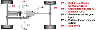
Crankshaft mounted electric machine (P1)

The P1 architecture, with the electric machine connected directly to the crankshaft, is the solution adopted by Honda on their first generation Integrated Motor Assist (IMA) technology. The electric motor functions as a generator, during vehicle deceleration, as an engine starter, and as a motor (to assist the engine) during vehicle accelerations.

Image: MHEV P1 architecture – Integrated Starter Generator (ISG)

One of the biggest advantage of this solution is that the electric motor can provide higher torque than the BiSG, since there is no belt limitation (due to slip). However, since there is no speed / torque ratio between the electric machine and crankshaft, the torque requirements on the electric motor can be quite demanding.

Two examples of P1 MHEV architectures are:

• Honda Insight Hybrid 2009 (with Integrated Motor Assist technology)
• Mercedes Benz S400 Bluehybrid 2010

Image: Integrated Motor Assist (IMA) for mild hybrid
Credit: Honda

For example, the main characteristics of the crankshaft-mounted electric machine for mild hybrid Honda Insight 2009 are summarized in the table below.

Electric machine performance	Maximum torque (at crankshaft): up to 34 Nm Maximum power: 10 kW Efficiency: up to 94%
Hybrid modes (functions)	Idle Stop & Start Moving Stop & Start Engine load shift Torque assist (fill) Torque boost Sailing / Coasting Energy recuperation Brake regeneration
Advantages	Higher efficiency The 12V starter can be removed
Disadvantages	Output torque limited by the size of the electric machine Energy recuperation affected by engine friction losses High impact on existing vehicle architecture Higher overall cost of the electrical components Air cooling not possible for the electric machine
Overall characteristics	Torque Boosting Capability: High (if electric machine is capable) Electrical Energy Recuperation: Medium (due to engine losses) Driveability Improvements: Medium (depending on the torque capability of the electric machine) Electrical Creep / Drive: Possible (depending on the torque capability of the e-machine) Packaging: Difficult components integration (powertrain specially designed for this architecture) System Efficiency: High (no gear mesh or belt losses)

Image: Mercedes Benz S400 BlueHybrid (MHEV)
Credit: Daimler

The primary advantage of a P1 mild hybrid architecture, compared with P0, is the removal of the belt drive. This means that the efficiency increases a bit (no more belt losses) and the electric machine torque can be higher in terms of amplitude and response (no more belt slip).

The functions (modes) performed by this mild hybrid topology are similar with those of a BiSG (P0), but, overall, P1 configurations have two big disadvantages: higher cost and higher impact on the the existing vehicle architecture. Therefore, vehicle manufacturers and system suppliers are not investing in the further development of crankshaft-mounted integrated starter generator solution for MHEV applications.

Model Structure :

There are two basic types of structure for the energy based models :

• Forward Model : Dynamic simulation of the system.
• Backward Model : Quasi-static simulation of the system.

Forward models simulate from the source to the sink viz. start simulation from the input to the engine to the wheels to determine the vehicle performance.

Backward models simulate from the source to the sink viz. input is the vehicle speed and acceleration, and the engine input is back calculated.

Forward Model :

• Forward models are a Dynamic Simulation.
• Dynamic models are used for detailed simulations.
• Force/torque/power is the input and the vehicle state variables velocity and acceleration are outputs.
• Models and simulation are more realistic due to physical causality, hence appropriate for control development.
• There is a feedback loop to meet the desired vehicle state.
• Slower simulation due to the dynamics.
• Approach mainly used to simulate a vehicle on a driving cycle, to analyse the dynamic behaviour of the system. Helps significantly in control development.

Matlab Script :

Matlab script used to load all the variables required for running the Simulink model and for post-processing. The drive cycle selection is also done here.

%% Initialization File
% Initialization file for loading the variables for the Conventional vehicle simulation model

%% Vehicle Parameters
M = 1500;       % Vehicle weight [kg]
Cr = 0.015;     % Rolling resistance coefficient
Rw = 0.35;      % Rolling radius [m]
Cd = 0.33;      % Drag coefficient
Af = 2;         % Frontal area [m2]
rhoa = 1.225;   % Air density [kg/m3]
Vwind = 0;      % Wind velocity [kmph]
g = 9.81;       % Gravitational acceleration [m/s2]
theta = 0;      % Slope [deg]
myu_road_tire = 1; % Coefficient of friction between tire - road interface

%% Powertrain Parameters 
FDR = 3.73;                         % Final Drive Ratio / Diff Ratio
DiffEff = 0.99;                     % Differential efficiency (assumed independent of operating conditions)

NumGear = 4;                        % Number of gears in transmission
TransGear = [1:NumGear];            % Transmission Gears
TransRatio = [3.06, 1.62, 1, 0.7];  % Corresponding Transmission ratios
TransEff = 0.90;                    % Transmission efficiency (assumed independent of operating conditions)

TC_SR = [0, .5, .6, .7, .8, .87, .92, .94, .96, .97, 1];   % Torque Converter Speed Ratio (Matlab default) -> TurbSpd/PumpSpd  
TC_TR = [2.232, 1.5462, 1.4058, 1.2746, 1.1528, 1.0732, 1.0192, 1, 1, 1, 1];   % Torque Converter Torque Ratio (Matlab default) -> TurbTrq/PumpTrq
TC_Cf = 1e-4 * [.72558, .66322, .63463, .59042, .51331, .4144, .29287, .22444, .12186, .04386, 0]; % Torque Converter Capacity Factor (Matlab default) -> PumpTrq/PumpSpd^2 [Nm/rpm^2]

load Vehicle_Data/Engine_data_1_9L_Saturn_95kW
load Vehicle_Data/Trans_Shift_map
load Vehicle_Data/EM_Honda_Insight_10kW
load Vehicle_Data/ESS_NiMH6


ESS_init_soc = 0.8;
ESS_soc_max = 0.9;
ESS_soc_min = 0.6;


%% Driver Parameters
Kp = 10;                    % P gain for driver PI model
Ki = 1;                     % I gain for driver PI model
Drive_Cycle_Select = 2;     % Drive cycle selection

% Drive cycle values in m/s

if Drive_Cycle_Select == 1
    load DriveCycles/UDDS;
    
elseif Drive_Cycle_Select == 2
    load DriveCycles/HWFET;
    
elseif Drive_Cycle_Select == 3
    load DriveCycles/FTP;
    
elseif Drive_Cycle_Select == 4
    load DriveCycles/US06;
    
elseif Drive_Cycle_Select == 5
    load DriveCycles/NEDC;
    
elseif Drive_Cycle_Select == 6
    load DriveCycles/WLTP;
 
end

time_end = cyc_time(end);
vel_end = cyc_vel(end);

While running this script in matlab the result showing in the workspace are as follows,

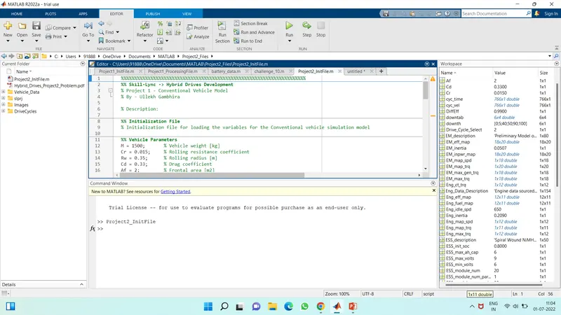
• After running the program all variables which are useful for run the simulink model are loaded in the workspace.
• The detailed simulink model for developement of P1 hybrid are shown below

Blocks used in Modelling :

Constant block :

The Constant block generates a real or complex constant value signal. Use this block to provide a constant signal input. The block generates scalar, vector, or matrix output, depending on: The dimensionality of the Constant value parameter.

GoTo :

Goto (Simulink Reference) The Goto block passes its input to its corresponding From blocks. The input can be a real- or complex-valued signal or vector of any data type. From and Goto blocks allow you to pass a signal from one block to another without actually connecting them.

Connection Port :

A subsystem needs a Connection Port block for each physical connection line that crosses its boundary. You can manually place a Connection Port block inside a subsystem, or Simulink can automatically insert a Connection Port block when you create a subsystem within an existing network.

PS Lookup Table :

A lookup table block uses an array of data to map input values to output values, approximating a mathematical function. Given input values, Simulink performs a “lookup” operation to retrieve the corresponding output values from the table.

Scope :

Scope, Floating Scope (Simulink Reference) The Scope block displays its input with respect to simulation time. The Scope block can have multiple axes (one per port); all axes have a common time range with independent y-axes. The Scope allows you to adjust the amount of time and the range of input values displayed.

Gain :

The Gain block multiplies the input by a constant value (gain). The input and the gain can each be a scalar, vector, or matrix. You specify the value of gain in the Gain parameter. The Multiplication parameter lets you specify element-wise or matrix multiplication.

Integrator :

Integrator (Simulink Reference) The Integrator block outputs the integral of its input at the current time step. The following equation represents the output of the block y as a function of its input u and an initial condition y ₀, where y and u are vector functions of the current simulation time t .

Saturation :

Saturation (Simulink Reference) The Saturation block imposes upper and lower bounds on a signal. When the input signal is within the range specified by the Lower limit and Upper limit parameters, the input signal passes through unchanged.

Dynamic Saturation :

The Saturation Dynamic block bounds the range of an input signal to upper and lower saturation values. An input signal outside of these limits saturates to one of the bounds where: The input below the lower limit is set to the lower limit. The input above the upper limit is set to the upper limit.

Rate limitor :

The Rate Limiter Dynamic block limits the rising and falling rates of the signal. The external signal up sets the upper limit on the rising rate of the signal. The external signal lo sets the lower limit on the falling rate of the signal.

Bus Creater :

The Bus Creator block combines a set of input elements into a bus. You can connect any element types to the input ports, including other buses. You can access elements in a bus by using a Bus Selector block. Elements of a bus must have unique names.

Bus Selector :

The Bus Selector block outputs the elements you select from the input bus. The block can output the selected elements separately or in a new virtual bus. The Bus Selector block does not support mixing message and signal elements as outputs.

Switch :

The Manual Switch block is a toggle switch that selects one of its two inputs to pass through to the output. To toggle between inputs, double-click the block. You control the signal flow by setting the switch before you start the simulation or by changing the switch while the simulation is executing.

Clock :

The Clock block outputs the current simulation time at each simulation step. This block is useful for other blocks that need the simulation time. When you need the current time within a discrete system, use the Digital Clock block. A Clock block outputs a real-valued signal of type double .

Vehicle Simulink Model :

Forward energy-based fuel consumption model of a P1 hybrid vehicle.

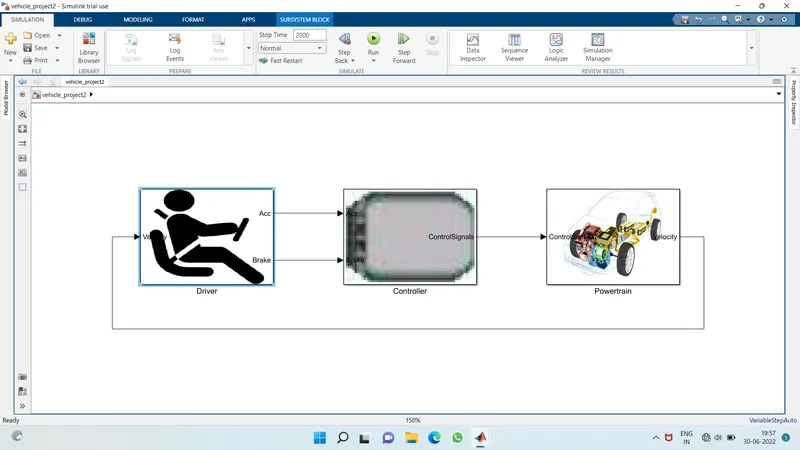
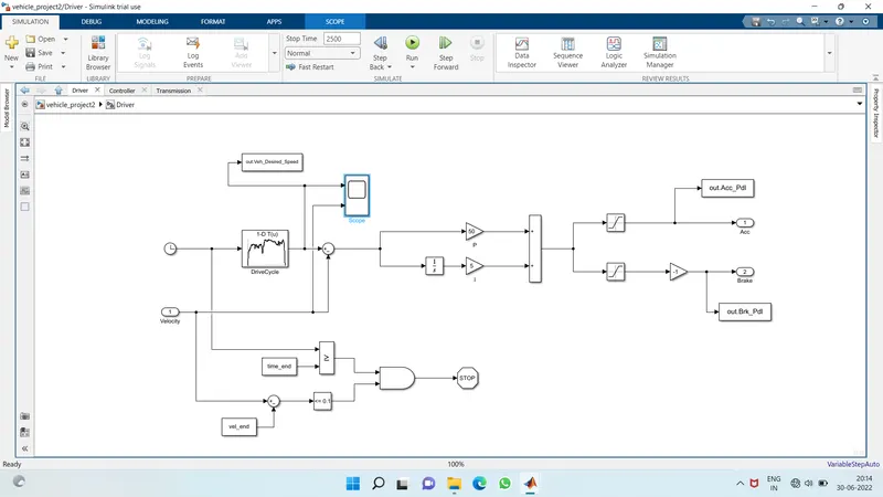
Driver Block :

• The Driver block which is a basic Pl controller that generates acc and brake pedal outputs to match the desired and actual vehicle speed.
• It uses a drive cycle, a drive cycle typically represented as a series data point which plots the vehicle speed against time.
• The vehicle desired speed is provided in the relational operatorand baloon condition based upon the simulation stop will execute.
• the sturation block limits the upper and lower condition based on the limit provides.

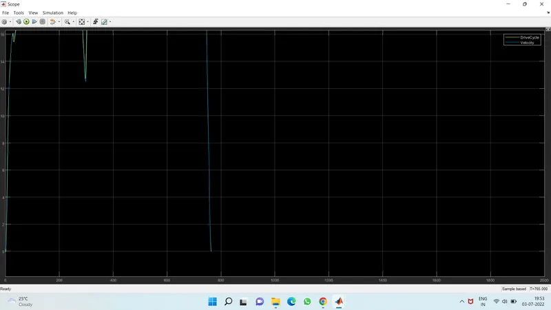
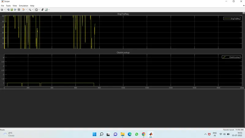
Scope Result :

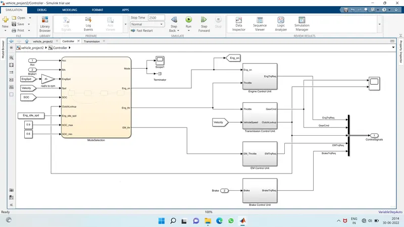
Controller Block :

• The controller block is the brain of the vehicle, representing the electronic controls unit. Based on the driver input , it generates desired engine torque, desired transmission gear and desired brake torque.
• It consist of Engine control unit, Transmission control unit, EM control unit and Brake control unit.
• This block are subsystems of the controller block.

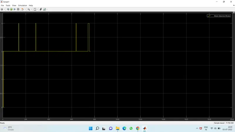
Scope Result :

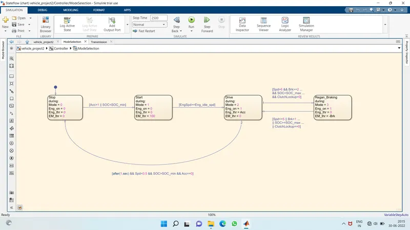
1. Stateflow chart of Mode Selection :

• The state flow chart consist of block as stop, start, drive and regen braking
• The operations like Mode, engine on, engine throttle are presents in the block
• The inputs are Acc, Brake, Velocity, SOC like that are mensioned
• Also Mode, Engine on, EM thr and Engine thr are the outputs.
• The block 1 and 2 are connected i.e. the command moves from 1 to 2
• In block 3 the engine is on and eng thr also positive but the EM thr is 0
• Block 4 shows the regen braking also it receives the negative power due to braking.

2. Engine Control Unit :

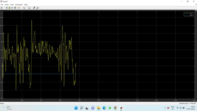
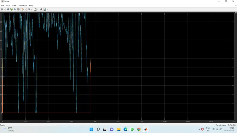
• The engine control unit derives the engine speed to execute the engine torque requirement.
• In the engine control unit the max and min torque are mapped by using 1-D lookup table and the signals are combined with the ideal speed controller.

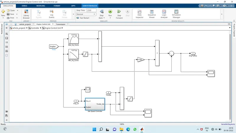
Scope Result :

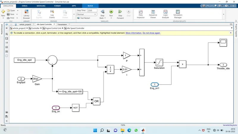
• Idle Speed Control unit :

1. It consist of mainly OR and NOT conditions block
2. The whole block maintain the idle speed of the engine.

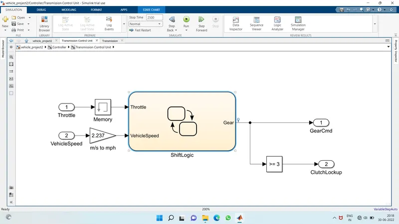
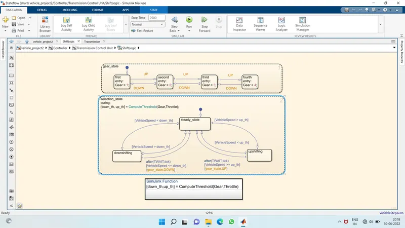
3. Transmission Control Unit :

• In the transmission control unit Trottle and vehicle speed are inputtes to the gear transmission logic control system.
• Based on the vehicle speed and throttle response the gears command are controlled.

• Gear Shift Logic Chart :

1. Based on the vehicle speed and throttle response the gears are selected based on the state and during conditions.
2. The up and down gears are shifted based upon the conditions and the actions on the logics.
3. Based on the simulink function using 2-D lookup table to map the up shifting and down shifting conditions.

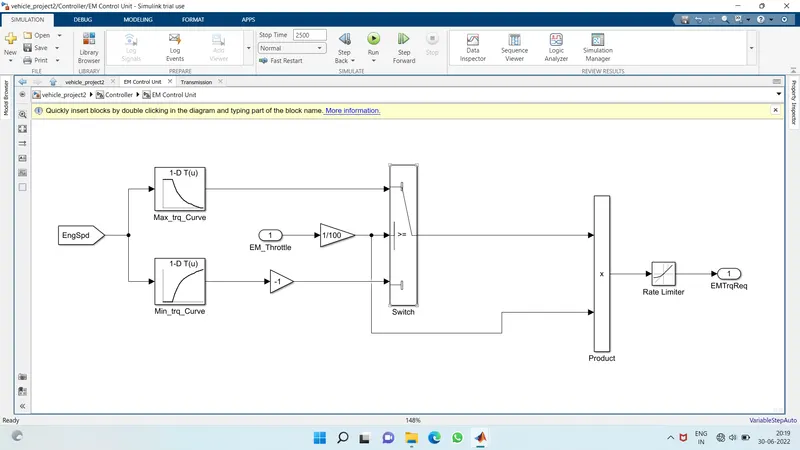
4. EM Control Unit :

• EM control unit is basicaly used as for electric motor control
• It consit of lookup table for give the input of max and min torque
• also gain, switch, product and main is rate limitor block used for simulation
• It controls the electric motor.

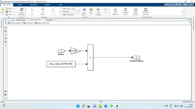
5. Brake Control Unit :

• The brake control unit is controlled on the mass, gravity, wheel radius and the coefficients of friction between the tire and the road surfaces.
• The brake and the tire load are multiply for finding the brake torque.

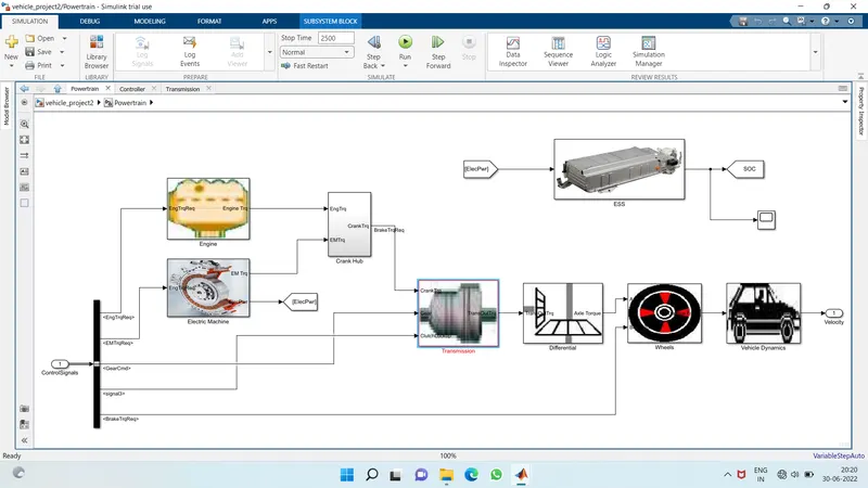
Powertrain Block :

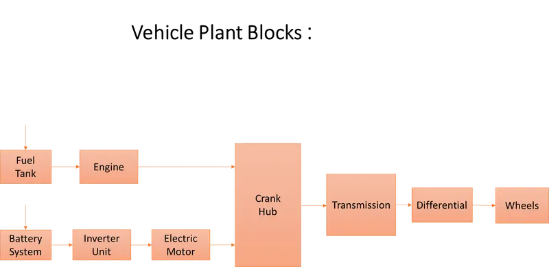
The powertrain block which represents the drivetrain of the vehicle. it consist of an Engine connected to the Automatic transmission through a torque converter. The output of the transmission is connected to the Differential, which powers the wheels, that provides the tractive force for vehicle acceleration. The longitudinal dynamics of the vehicle along with the road load is represented in the vehicle dynamic block.

1. Engine Block Model :

• The engine model is modelled using the engine speed and engine torque requirement.
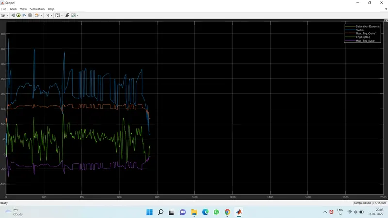
• Based on the engine torque and engine speed the max and min torque are mapped using 1-D look up table and that are saturated using upper and lower limits.
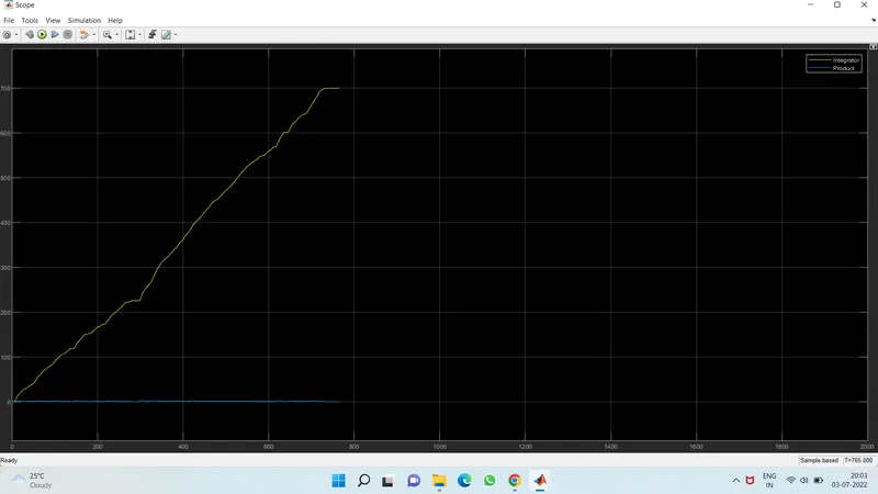
• The saturated executes the engine fuel rate and the integration of the fuel flow rate gives the fuel consumption of the engine.

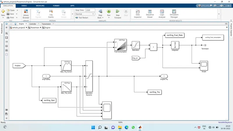
Scope Result :

2. Electric Machine :

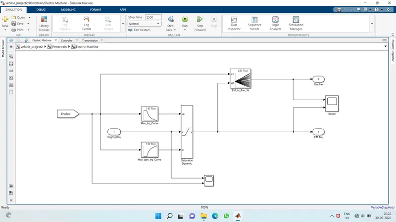
Scope Result :

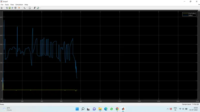
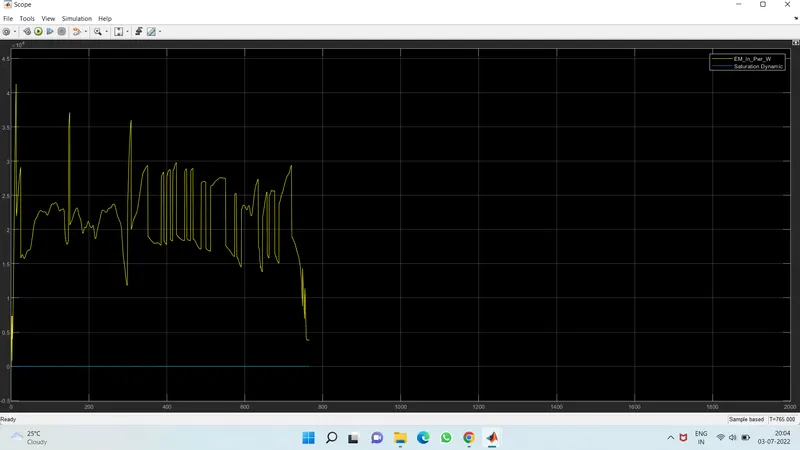
3. Crank Hub :

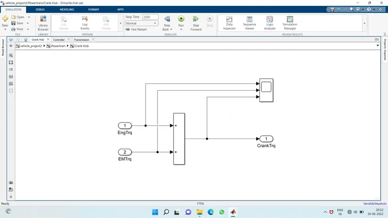
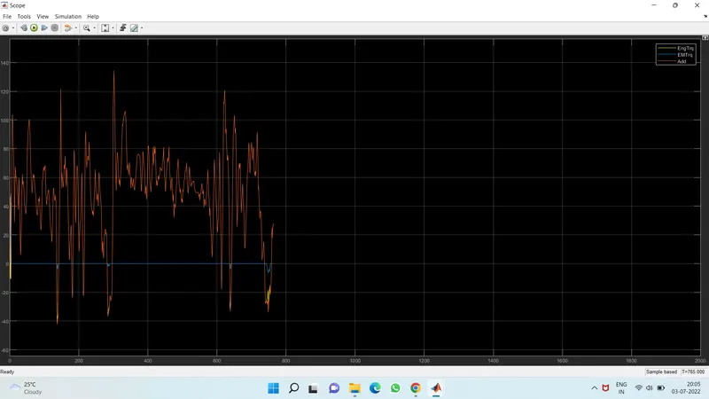
Scope Result :

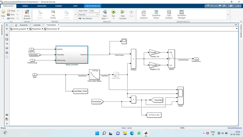
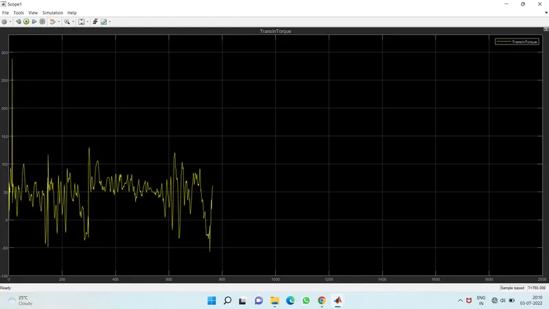
4. Transmission Block Model :

• The engine torque and the gear transmiossion are inputted into the transmission block.
• Based upon the transmission input torque and transmission output speed the positive and negative effeciencies are determined using switch threshold conditions.
• From which the transmission output torque are derived.

Scope Result :

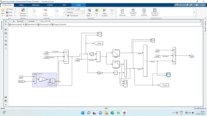
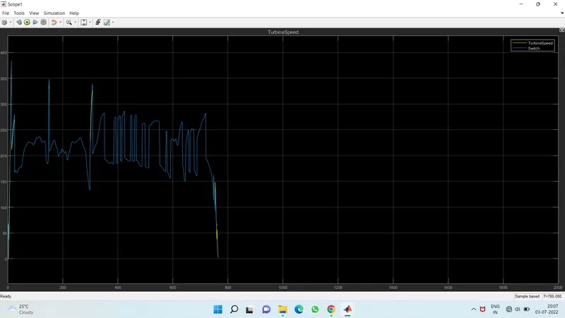
• Torque Converter :

1. In the torque converter the pump and turbine torque are determined by using the 1-D mapped models.
2. The pump torque are derived by using the c-factor mapped 1-D model.

Scope Result :

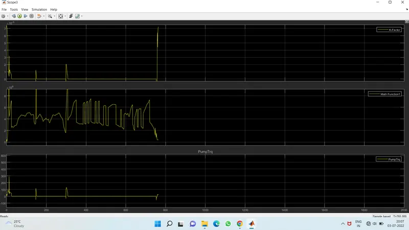
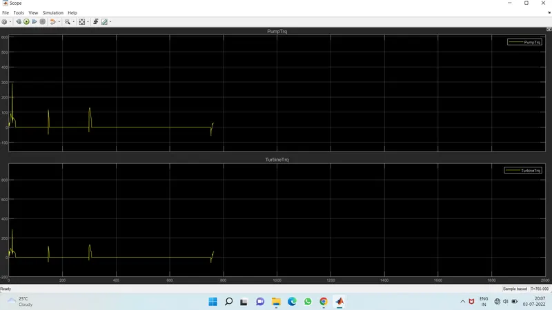
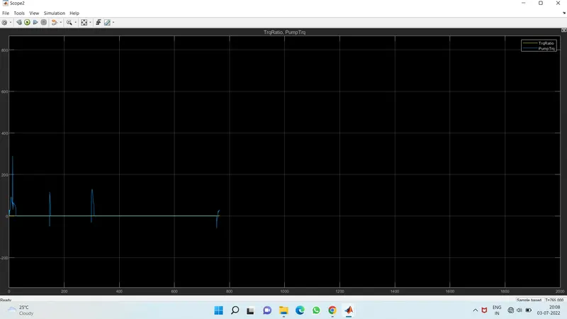
5. Differential Block Model :

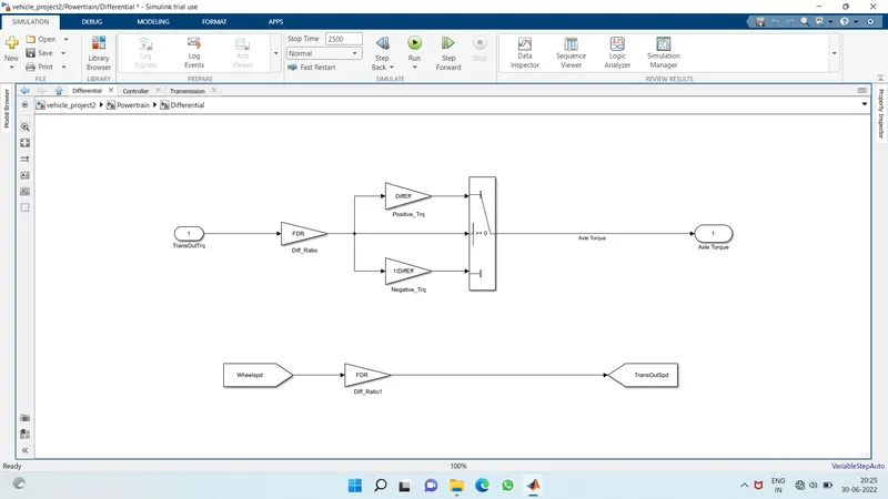
• The transmission output torque is inputed into the gain of final drive ratio by which the positive and negative differential efficiencies are derived by using switch threshold conditions
• The wheel speed from thye vehicle is inputted to compute the transmission output speed.

6. Wheel Model Block :

• The net torque axle torque and brake torque are transmitted into the wheel and the wheel radius are determined to estimate the tractive force.
• The wheel speed is determined by using the velocity of the vehicle and te wheel radius.

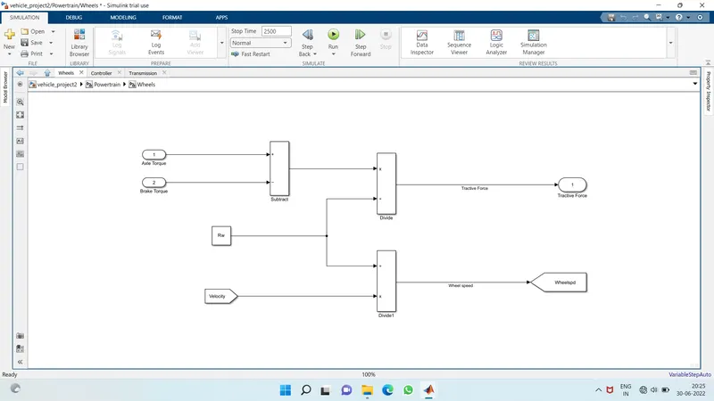
7.Vehicle Dynamics :

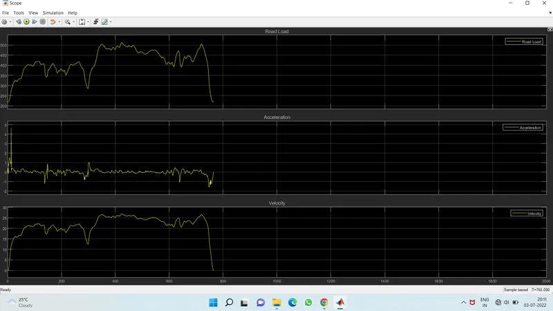
The vehicle dynamics is the motion of the vehicle generated by the steering action, through which the vehicle is capable of independent motion, in a vehicle several forces act on it and the net or resultant force governs the motion according to the newtons second law.

The propulsion unit of the vehicle delivers the forces neccesary to move the vehicle forward. This force of the propulsion unit helps the vehicle to overcome the resisting forces due to gravity, air and tire resistance.

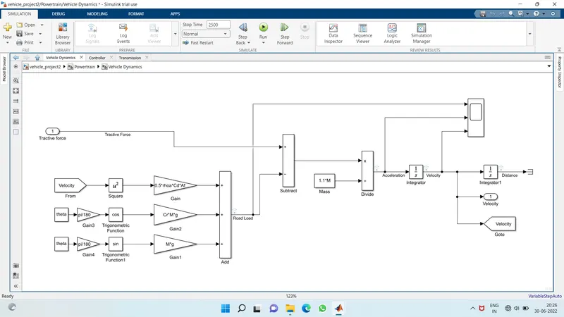
Scope Result :

Battery Modelling :

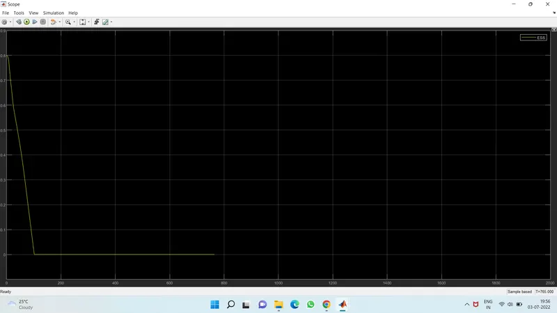
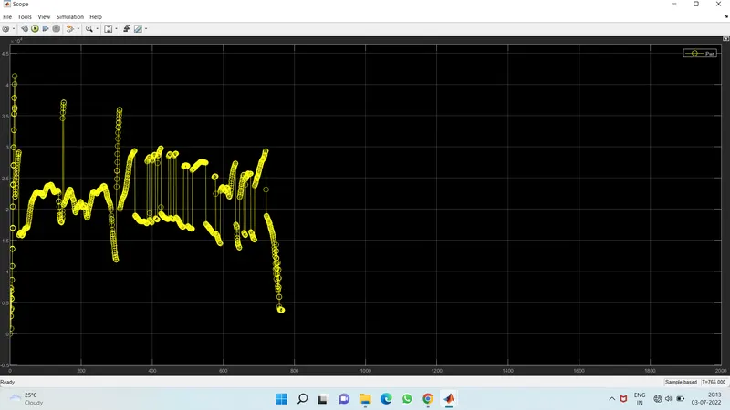
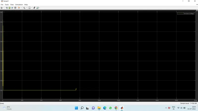
1. ESS (Estimated Storage System)

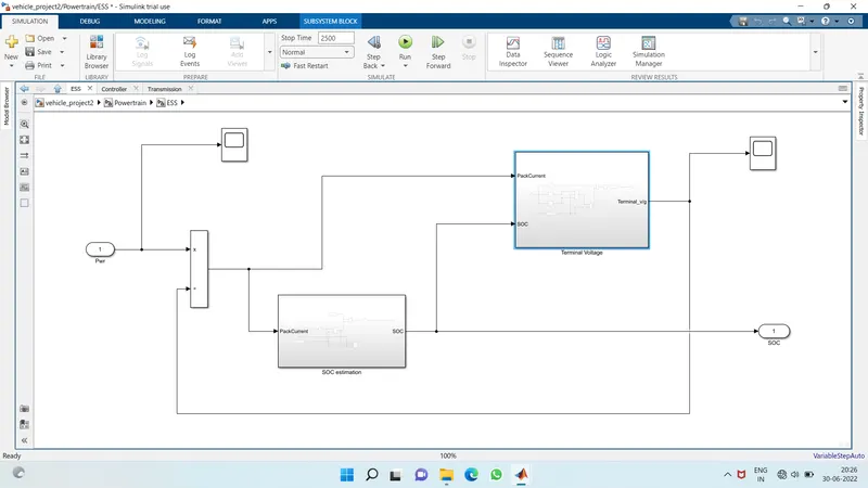
Scope Result :

2. Terminal Voltage :

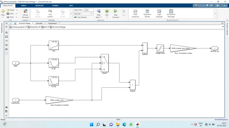
3. SOC Estimation :

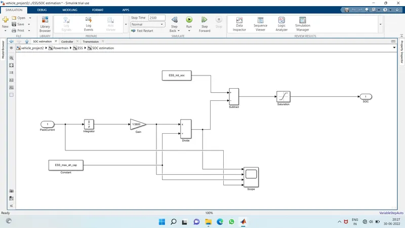
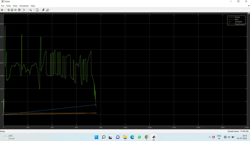
Scope Result :

Matlab Script for Post Processing File :

%%%%%%%%%%%%%%%%%%%%%%%%%%%%%%%%%%%%%%%%%%%%%%%%%%%%%%%%%%%%%%%%%%%%%
%% Skill-Lync -> Hybrid Drives Development
% Project 1 - Conventional Vehicle Model
% By - Ullekh Gambhira 

% Description:
% The following file is to used with the Initialization file and Simulink
% results for post-processing of the data.
% The file is incomplete, has some examples of how the data is imported
% into a readable format, data analysis and plotting examples.
% Based on the project task, use commands in a similar format as given
% below, to analyse the data and generate required plots.
% You can change variable names if desired

%% Post-Processing File
%  File for post-processing the Conventional vehicle simulation model data

%% Renaming variables
Time = out.tout;
Acc_Pdl = out.Acc_Pdl;          % Accelerator pedal [%]
Brk_Pdl = out.Brk_Pdl;          % Brake pedal [%]
Gear_Cmd = out.Gear_Cmd;        % Transmission gear
Trans_In_Spd = out.Trans_In_Spd*30/pi;  % Transmission input speed [rpm]
Trans_Out_Spd = out.Trans_Out_Spd*30/pi;% Transmission output speed [rpm]
Eng_Trq = out.Eng_Trq;          % Engine brake torque [Nm]
Eng_Spd = out.Eng_Spd*30/pi;    % Engine speed [rpm]
Eng_Fuel_Rate = out.Eng_Fuel_Rate; % Engine Fuel Rate
Eng_Fuel_Consump = out.Eng_Fuel_Consumption;    % Engine fuel consumption [g]
Veh_Dist = out.Veh_Dist/1000;   % Distance traveled by vehicle [km]
Veh_Spd = out.Veh_Spd*18/5;     % Vehicle speed [kmph]
Desired_Spd = out.Desired_Spd*18/5;  %Desired Speed (Kmph)
Wheel_Spd = out.Wheel_Spd*30/pi;     %Wheel speed (rpm)

%% Data Analysis
Eng_Pwr = Eng_Spd*pi/30*Eng_Trq/1000;   % Engine brake power [kW]
rho_petrol = 0.7197;                    % Density of petrol [kg/L]
Veh_Distance = (out.Veh_Dist.Data(:,1))/1000;
Eng_Fuel_Consumption = out.Eng_Fuel_Consumption.Data(:,1);
kmpl = Veh_Distance(end)/(Eng_Fuel_Consumption(end)/1000/rho_petrol);    % Fuel economy [kmpl] 

%% Fuel Economy For Engine 
T = table({'FUEL ECONOMY'},(kmpl));
T.Properties.VariableNames = {'ENGINE','KMPL'}
writetable(T,'UDDS.xlsx','Sheet',1);

%%Plotting
%%Plotting the drive cycle
figure(1)
plot(cyc_time,cyc_vel,'LineWidth',2,'Color','r')
grid on
xlabel('Time[sec]')
ylabel('Velocity[Mph]')
legend('Drive Cycle')

%% Plotting for the time trace for engine
figure(2)
hold on
plot(Time, Acc_Pdl, 'linewidth', 1, 'Color', 'b');
plot(Time, Brk_Pdl, 'linewidth', 1, 'Color', 'g');
plot(Wheel_Spd,'LineWidth',1,'Color','black')
grid on
xlabel('Time[sec]')
ylabel('Speed[rpm]')
legend('Transinspeed - Transoutspeed - Wheelspd')
title('Time Trace for Engine')


%% Plotting vehicle characteristics time trace
figure(3)
subplot(3,1,1)
hold on
grid on
plot(Time, Acc_Pdl, 'linewidth', 1, 'Color', 'black');
plot(Time, Brk_Pdl, 'linewidth', 1, 'Color', 'red');
xlabel('Time[sec]')
ylabel('Pedal [%]')
xlim([0, Time(end)]);
title('Acc and Brk Padel')
legend('Accel','Brake');
subplot(3,1,2)
hold on
grid on
plot(Desired_Spd, 'linewidth', 1, 'Color', 'black');
plot(Veh_Spd, 'linewidth', 1, 'Color', 'red');
xlabel('Time[sec]')
ylabel('Speed [rpm]')
title('Desired and Actual Speed')
legend('Trans Input','Trans Output');
subplot(3,1,3)
hold on
grid on
plot(Time, Gear_Cmd, 'linewidth', 1, 'Color', 'g');
xlim([0, Time(end)]);
xlabel('Time [s]');
ylabel('Gear');
title('Gear Command')
legend('Gear')


%% Plotting engine operating points on engine fuel map
figure('Name','Engine Operating Points');
hold on
grid on
title('Engine Operating Points','fontsize',12);
p1=plot(Eng_map_spd*30/pi,Eng_max_trq,'linewidth',2,'color','r');
p2=line([Eng_map_spd(end)*30/pi Eng_map_spd(end)*30/pi],[0 Eng_max_trq(end)]);
set(p2,'linewidth',1,'linestyle','--','color','k');
p3=line([Eng_map_spd(1)*30/pi Eng_map_spd(1)*30/pi],[0 Eng_max_trq(1)]);
set(p3,'linewidth',1,'linestyle','--','color','k');
[c,h] = contour(Eng_map_spd'*30/pi,Eng_map_trq,Eng_fuel_map');
clabel(c,h);
xlabel('Engine Speed [rpm]');
ylabel('Engine Torque [Nm]');
title('Engine Fuel Consumption Map [g/s]');
p4 = plot(Eng_Spd,Eng_Trq,'.','color','k');
legend([p1 p4],{'Max Curve','Operating Points'});
axis([Eng_map_spd(1)*30/pi Eng_map_spd(end)*30/pi 0 Eng_map_trq(end)]);

RESULTS :

Plot Result :

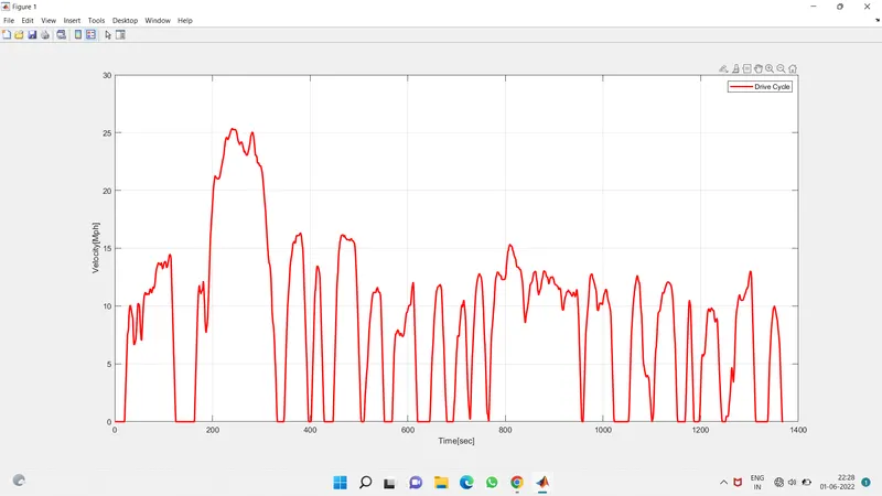
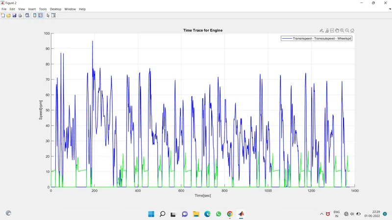
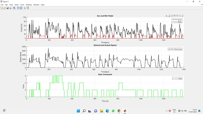
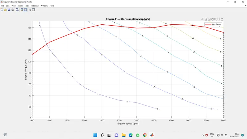
Result :

Fuel Economy

• For UDDS drive cycle is 15.0773
• For HWFET drive cycle is 17.1613

As we see the fuel economy numbers for project 2 are bit higher than the project 1 because of implementing the electric motor as it is P1 hybrid it may not have much variation in the fuel economy but as we implement other architecture it will increase by huge amount.