Week 4.1 - Genetic Algorithm
Question : Explain the concept of Genetic Algorithm ?
Ans - A genetic algorithm (GA) is a method for solving both constrained and unconstrained optimization problems based on a natural selection process that mimics biological evolution. The algorithm repeatedly modifies a population of individual solutions. also A genetic algorithm is a search heuristic that is inspired by Charles Darwin's theory of natural evolution. This algorithm reflects the process of natural selection where the fittest individuals are selected for reproduction in order to produce offspring of the next generation.
Five phases are considered in a genetic algorithm:
- Initial population
- Fitness function
- Selection
- Crossover
- Mutation
Question : Explain the syntax for ga in MATLAB ?
Ans -
x= ga(fun,nvars)x, to the objective function,fun.nvarsis the dimension (number of design variables) offun.
x= ga(fun,nvars,A,b)xtofun, subject to the linear inequalitiesA*x≤b.gaevaluates the matrix productA*xas ifxis transposed (A*x')
x= ga(fun,nvars,A,b,Aeq,beq)xtofun, subject to the linear equalitiesAeq*x=beqandA*x≤b. (SetA=[]andb=[]if no linear inequalities exist.)gaevaluates the matrix productAeq*xas ifxis transposed (Aeq*x').
x= ga(fun,nvars,A,b,Aeq,beq,lb,ub)x, so that a solution is found in the rangelb≤x≤ub. (SetAeq=[]andbeq=[]if no linear equalities exist.)
x= ga(fun,nvars,A,b,Aeq,beq,lb,ub,nonlcon)nonlcon. The functionnonlconacceptsxand returns vectorsCandCeq, representing the nonlinear inequalities and equalities respectively.gaminimizes thefunsuch thatC(x)≤0andCeq(x) = 0. (Setlb=[]andub=[]if no bounds exist.)
x= ga(fun,nvars,A,b,Aeq,beq,lb,ub,nonlcon,options)options. (Setnonlcon=[]if no nonlinear constraints exist.) Createoptionsusingoptimoptions.-
x= ga(fun,nvars,A,b,Aeq,beq,lb,ub,nonlcon,intcon)x= ga(fun,nvars,A,b,Aeq,beq,lb,ub,nonlcon,intcon,options)intcontake integer values.
[, for any previous input arguments, also returnsx,fval] = ga(___)fval, the value of the fitness function atx.
[also returnsx,fval,exitflag,output] = ga(___)exitflag, an integer identifying the reason the algorithm terminated, andoutput, a structure that contains output from each generation and other information about the performance of the algorithm.
[also returns a matrixx,fval,exitflag,output,population,scores] = ga(___)population, whose rows are the final population, and a vectorscores, the scores of the final population.
Program for stalagmite Function :
function [A]= stalagmite_func(input_vector)
x=input_vector(1);
y=input_vector(2);

a1=(sin(5.1*pi*x+0.5))^6;
a2=exp(-4*log(2)*(x-0.0667)^2/0.64);
a3=(sin(5.1*pi*y+0.5))^6;
a4=exp(-4*log(2)*(y-0.0667)^2/0.64);

[A]=-(a1*a2*a3*a4)

end
Program for Study1- Statistical Behaviour
clear all
close all
clc

% defining our search space
x=linspace(0,0.6,150);
y=linspace(0,0.6,150);
num_cases=50;
[xx, yy]= meshgrid(x,y);

% evaluating the stalagmite function
for i=1:length(xx)
    for j=1:length(yy)
        input_vector(1)=xx(i,j);
        input_vector(2)=yy(i,j);
        f(i,j)=stalagmite_func(input_vector);
    end
end

tic
%study one statistical behavior
for i=1:num_cases
    [inputs,fopt(i)]=ga(@stalagmite_func,2);
    xopt(i)=inputs(1);
    yopt(i)=inputs(2);
end
study1_time=toc

figure(1)
subplot(2,1,1)
hold on
surfc(xx,yy,-f)
shading interp
plot3(xopt,yopt,-fopt,'Marker','o','MarkerSize',5,'MarkerFaceColor','r')
title('unbounded inputs')
subplot(2,1,2)
plot(-fopt)
xlabel('Iterations')
ylabel('function minimum')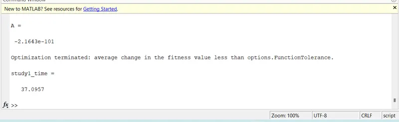
tic
% study two Statistical behaviour with upper and lower bounds
for i=1:num_cases
    [inputs, fopt(i)]=ga(@stalagmite_func,2,[],[],[],[],[0;0],[1;1]);
    xopt(i)=inputs(1);
    yopt(i)=inputs(2);
end
study2_time=toc

figure(2)
subplot(2,1,1)
hold on
surfc(xx,yy,-f)
shading interp
plot3(xopt,yopt,-fopt,'Marker','o','MarkerSize',5,'MarkerFaceColor','r')
title('unbounded inputs')
subplot(2,1,2)
plot(-fopt)
xlabel('Iterations')
ylabel('function minimum')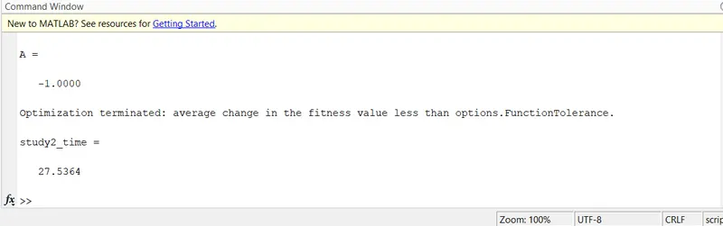
Program for study3- Increasing GA Iterations :
% study three increasing GA iterations
options=optimoptions('ga')
options=optimoptions(options,'PopulationSize',170)
tic
for i=1:num_cases
    [inputs,fopt(i)]=ga(@stalagmite_func,2,[],[],[],[],[0;0],[1;1],[],[],options);
    xopt(i)=inputs(1);
    yopt(i)=inputs(2);
end
study3_time=toc

figure(3)
subplot(2,1,1)
hold on
surfc(xx,yy,-f)
shading interp
plot3(xopt,yopt,-fopt,'Marker','o','MarkerSize',5,'MarkerFaceColor','r')
title('unbounded inputs')
subplot(2,1,2)
plot(-fopt)
xlabel('Iterations')
ylabel('function minimum')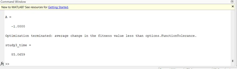
- clear all close all and clc is used for clear and close the data in command and workspace window
- linspace is used for create an 2D array
- meshgrid is used for 3d array
- function code is used for create a limit loop
- plot command plots the data
- subplot create divide a plot in 2 parts
- hold command holds the plot
- surfc creats 3D surface plot
- shading interp is use for remove the lines on figure
- title creates the name of plot
- xlabel and ylabel are for naming the axis
- marker is used for creat the point
- markersize code is for how the point in size
- markerfacecolor shows the color of the points.