Project 2 - Rankine cycle Simulator

Rankine Cycle Simulator

Aim : Create a Rankine Cycle Simulator by using GNU Octave.

Objectives :

1. Calculate the state points of the Rankine Cycle
2. Plot the corresponding T-s and h-s plots for the given set of inputs. Title and axes labels are a must, while legends could be used if necessary.
3. Calculate Efficiency.

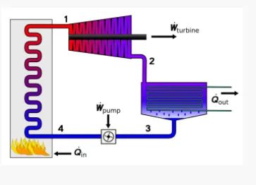
Basic Rankine cycle image for study :

Theory :

The ideal rankine cycle consist of the following 4 processes as shown in the below result from the above fig.

• 1-2 : Isentropic expansion in the turbine
• 2-3 : constant pressure and heat rejection in the condenser
• 3-4 : Isentropic compression in the compressor
• 4-1 : constant pressure and heat additionin the boiler.

Explanation,

Turbine(process 1-2): the generated steam in the boiler which is high in tempreture and pressure is passed towards the turbine whenever process finishes the low pressure stem os passed towards the condenser, the energy balance in the turbine is, Wturbine, out = h2-h1

Condenser(process 2-3): the low pressure and tempretured steam form the turbine is entered in the condenser the tempreture cools down and steam is converted in the condenser, the energy balance in the condenser is,

Qout = h3-h2

Compressor(process 3-4): the condensed liquid is pass towards the pump and the liquid getting compressed in the compressor and passed towards boiler, the energy balance in the pump is,

Wpump, in=h4-h3

Boiler(process 4-1): the highly compressed liquid is passed in the boiler which is constant in pressure and the process of heat addition is being started and tempreture getting increased in the boiler and compressed liquid is converted in the high pressure and tempretured steam, the energy balance in the boiler is,

Qin = h1-h4

The program for Rankine Cycle is as follows :

main code -

clear all
close all
clc

%user inputs
fprintf('%75s','Rankine Cycle Simulator');
fprintf('nnn');
fprintf('1-2 is isentropic expansion in the turbine');
fprintf('2-3 is constant pressure and heat rejection by the condenser');
fprintf('3-4 is isentropic compression in the pump');
fprintf('4-1 is constant pressure and heat addition in the boiler');

%inputs
p1= input('Enter the pressure(in bar)at the inlet of the turbine(at point 1):');
t1= input('Enter the tempreture(in degree)at the inlet of the turbine(at point 1):');
p2= input('Enter the pressure(in bar)at the inlet of the condenser(at point 2):');


%inputs to the turbine
s1= Xsteam('s_pT',p1,t1);
h1= Xsteam('h_pT',p1,t1);

%condenser inlet
s2=s1

%1-2 process
sf2=Xsteam('sL_p',p2);
sg2=Xsteam('sV_p',p2);
hf2=Xsteam('hL_p',p2);
hg2=Xsteam('hV_p',p2);

%calculating dryness fraction
if (s2<=sg2)
   x2=((s2-sf2)/(sg2-sf2)); %Dryness Fraction at state point 2
else
   x2=1;
end

h2=hf2+(x2*(hg2-hf2));

%condenser exit
p3=p2;
t3=Xsteam('Tsat_p',p3);
s3=Xsteam('sL_p',p3);
h3=Xsteam('hL_p',p3);
v3=Xsteam('vL_p',p3);
t2=t3;

%boiler inlet
p4=p1; %constant pressure heat addition
s4=s3; %isentropic compression in the pump
h4=Xsteam('h_ps',p4,s4);
cp4=Xsteam('cp_ps',p4,s4);
cv4=Xsteam('cv_ps',p4,s4);
g4=(cp4/cv4);

%calculating for t4
%p4^(1-gamma)*t4^gamma=p3^(1-gamma)*t3^gamma;
t4=(t3*((p3/p4)^((1-g4)/g4)));

%calculation
%work done by turbine
wt=h1-h2;
%work done by turbine
wp=h4-h3;
%net work done
w_net=wt-wp;
%heat added in the boiler
q_in=h1-h4;
%heat rejection in the condenser
q_out=h2-h3;
%thermal efficiency
n=(w_net/q_in)*100;

%plotting the results
figure(1)
%plotting liquid and vapour curve
t=linspace(1,t1,1000);
for i= 1:length(t)
    s_l(i)=Xsteam('sL_T',t(i));
end

for i=1:length(t)
    s_v(i)=Xsteam('sV_T',t(i));
end
hold on
plot(s_l,t,'linewidth',2,'linestyle','- -','color','r');
plot(s_v,t,'linewidth',2,'linestyle','- -','color','r');
grid on

%plotting for the work done by the turbine(process 1-2)
plot([s1,s2],[t1,t2],'linewidth',2,'color','g')
hold on
title('T-S Diagram of Ideal Rankine Cycle')
xlabel('Entropy (KJ/KgK)')
ylabel('Tempreture(k)')

%plotting for the heat rejection in the condenser(process 2-3)
plot([s2,s3],[t2,t3],'linewidth',2,'color','g')
hold on

%plotting for the work done by the pump(process 3-4)
plot([s3,s4],[t3,t4],'linewidth',2,'color','g')
hold on

%plotting for the heat added by the boiler(process 4-1)
tp=Xsteam('Tsat_p',p4);
sp=Xsteam('sL_T',tp);
plot([s4,sp],[t4,tp],'linewidth',2,'color','g')
hold on

tq=tp;
sq=Xsteam('sV_T',tq);
plot([sp,sq],[tp,tq],'linewidth',2,'color','g')
hold on

plot([sq,s1],[tq,t1],'linewidth',2,'color','g')
hold on

%Indicate states with numbers
text(s1,t1,' 1');
text(s2,t2,' 2');
text(s3,t3,' 3');
text(s4,t4,' 4');

%plot for enthalpy vs entropy
figure(2)
plot([s1,s2],[h1,h2],'linewidth',2,'color','g')
grid on
title('h-s Diagram')
xlabel('Entropy (KJ/KgK)')
ylabel('Enthalpy(kJ/Kg)')
hold on

plot([s2,s3],[h2,h3],'linewidth',2,'color','g')
hold on
plot([s3,s4],[h3,h4],'linewidth',2,'color','g')
hold on
plot([s4,s1],[h4,h1],'linewidth',2,'color','g')

%Plot for liquid and vapour saturation curve

t=linspace(1,t1,1000);
for j= 1:length(t)
    h_l(j)=Xsteam('hL_T',t(j));
end

for j=1:length(t)
    h_v(j)=Xsteam('hV_T',t(j));
end

plot(s_l,h_l,'linewidth',2,'linestyle','- -','color','r');
hold on
plot(s_v,h_v,'linewidth',2,'linestyle','- -','color','r');
grid on

%Indicate states with numbers
text(s1,h1,' 1');
text(s2,h2,' 2');
text(s3,h3,' 3');
text(s4,h4,' 4');


%Result Output

fprintf('%40s n n n','RESULT');
fprintf('%10s %54s n','at state point 1','at state point 2');
fprintf('%s %.2f%s %44s %.2f%s n','P1:',p1,'bar','P2:',p2,'bar');
fprintf('%s %.2f%s %35s %.2f%s n','T1:',t1,'Deg Celcius','T2:',t2,'Deg Celcius');
fprintf('%s %.2f%s %40s %.2f%s n','H1:',h1,'KJ/Kg','H2:',h2,'KJ/Kg');
fprintf('%s %.2f%s %42s %.2f%s n','S1:',s1,'KJ/Kgk','S2:',s2,'KJ/Kgk');
fprintf('%58s %.2f n n','X2:',x2);
fprintf('%10s %54s n','at state point 3','at state point 4');
fprintf('%s %.2f%s %45s %.2f%s n','P3:',p3,'bar','P4:',p4,'bar');
fprintf('%s %.2f%s %35s %.2f%s n','T3:',t3,'Deg Celcius','T4:',t4,'Deg Celcius');
fprintf('%s %.2f%s %41s %.2f%s n','H3:',h3,'KJ/Kg','H4:',h4,'KJ/Kg');
fprintf('%s %.2f%s %42s %.2f%s n n','S3:',s3,'KJ/Kgk','S4:',s4,'KJ/Kgk');

fprintf('40%s %.2f%s %s n','work output by turbine(Wt):',wt,'KJ/Kg');
fprintf('40%s %.2f%s %s n','work input by pump(Wp):',wp,'KJ/Kg');
fprintf('40%s %.2f%s %s n','net work(Wnet):',w_net,'KJ/Kg');
fprintf('40%s %.2f%s %s n','Thermodynamics Efficiency(Ntherm):',n,'percent');
fprintf('40%s %.2f%s %s n','heat input in boiler:',q_in,'KJ/Kg');
fprintf('40%s %.2f%s %s n','heat rejection in condenser:',q_out,'KJ/Kg');
fprintf('40%s %.2f%s %s n','s.s.c.:',p3,'Kg/Kwh')

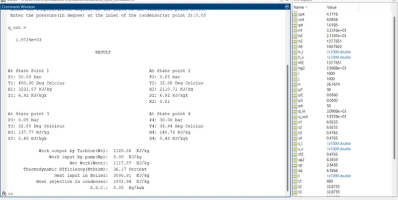
Obtained Output