Unsupervised and Supervised Model Building on Automobile 1985 dataset

Aim :

• To implement clustering using an unsupervised algorithm on the car dataset
• Train a supervised model from the results obtained to predict the class of the cars

Dataset :

The dataset is about cars from 1985, It consists of:

Number of Instances: 205

Number of Attributes: 26 total

• 15 continuous
• 1 integer
• 10 nominal

The following data was cleaned and feature selection and feature engineering were performed and we ended up with

Number of Instances: 201

Number of Attributes: 21

Methods :

Clustering

Clustering is performed using the KMeans algorithm, to find the right amount of clusters, the elbow plot is plotted

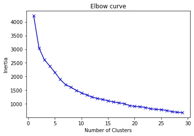
From the above plot, we can see that after 7 clusters the change in Inertia is very less, hence we go with 7 clusters

Results obtained from clustering

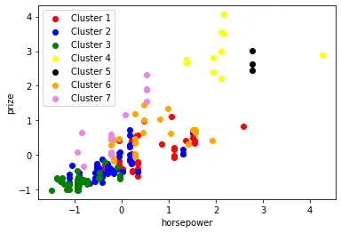
Cluster plot with respect to horsepower

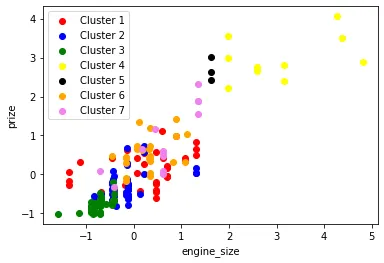
Cluster plot with respect to engine size

Classification using SVM

Now the output from the clustering is used to train a supervised model, we use the support vector machine algorithm(SVM) for this purpose

Results obtained from SVM

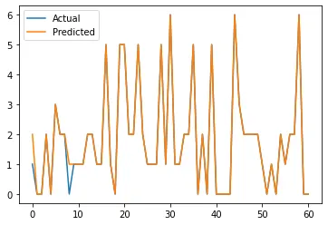
Plot between actual and predicted values

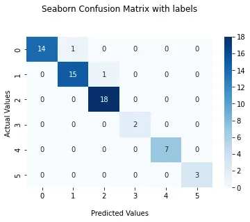
The confusion matrix is also visualized

Code :

import pandas as pd
import numpy as np
import matplotlib.pyplot as plt
import seaborn as sns
from sklearn.preprocessing import StandardScaler

#Assign names to each column
column_name=['symboling','normalized_losses','make','fuel','aspiration','num_of_doors','body_style','drive_wheels','engine_location','wheel_base','length','width','height','curb_weight','engine_type','num_of_cylinders','engine_size','fuel_system','bore','stroke','compression_ratio','horsepower','peak_rpm','city_mpg','highway_mpg','price']

#Read dataset
df=pd.read_csv('auto.csv',names = column_name)
print(df.columns)

print(df.info())
print(df.shape)
print(df.head())

# Replacing ? with NAN
df.replace("?",np.nan,inplace=True)
print(df.head())

#Converting datatype
#pd.set_option('display.max_columns', None)
df['normalized_losses']=df['normalized_losses'].astype(float)
df['bore']=df['bore'].astype(float)
df['stroke']=df['stroke'].astype(float)
df['horsepower']=df['horsepower'].astype(float)
df['peak_rpm']=df['peak_rpm'].astype(float)
df['price']=df['price'].astype(float)

print(df.describe())

#Finding total null values
print(df.isna().sum())

#Dealing with null values

#Replacing with mean values
df['normalized_losses'].replace(np.nan, 122,inplace=True)
df['bore'].replace(np.nan, 3.329050,inplace=True)
df['stroke'].replace(np.nan, 3.258300,inplace=True)
df['horsepower'].replace(np.nan, 104.222772,inplace=True)
df['peak_rpm'].replace(np.nan, 5125.990099,inplace=True)

#Replacing with highest frequency values
print(df['num_of_doors'].value_counts())
df['num_of_doors'].replace(np.nan, 'four',inplace=True)

#Dropping values
df.dropna(subset=["price"], axis=0, inplace=True)
df.reset_index(drop=True, inplace=True)
print(df.head())


#Feature engineering
df['fuel']=pd.get_dummies(df['fuel'],drop_first=True)

df['aspiration']=pd.get_dummies(df['aspiration'],drop_first=True)

df['num_of_doors']=pd.get_dummies(df['num_of_doors'],drop_first=True)

df['engine_location']=pd.get_dummies(df['engine_location'],drop_first=True)

df['num_of_cylinders'].replace('two', 2,inplace=True)
df['num_of_cylinders'].replace('three', 3,inplace=True)
df['num_of_cylinders'].replace('four', 4,inplace=True)
df['num_of_cylinders'].replace('five', 5,inplace=True)
df['num_of_cylinders'].replace('six', 6,inplace=True)
df['num_of_cylinders'].replace('eight', 8,inplace=True)
df['num_of_cylinders'].replace('twelve', 12,inplace=True)
df['num_of_cylinders']=df['num_of_cylinders'].astype(int)

gd = pd.get_dummies(df['drive_wheels'], prefix='dw_',drop_first=True)
df = pd.merge(left=df,right=gd,left_index=True,right_index=True)

#sns.boxplot(x="body_style", y="price", data=df)
#sns.boxplot(x="engine_type", y="price", data=df)
#sns.boxplot(x="fuel_system", y="price", data=df)

#Dropping unwanted features
df=df.drop(['make','drive_wheels','engine_type','fuel_system','body_style'],axis=1)
print(df.info())


#Corelation matrix
corr=df.corr().index
#plt.figure(figsize=(20,20))
#sns.heatmap(df[corr].corr(),annot=True,cmap='RdYlGn')

#Dropping highly corelated features
df=df.drop(['highway_mpg','compression_ratio'],axis=1)
print(df.info())
print(df.shape)

#Standardizing the data
sc=StandardScaler()
df=sc.fit_transform(df)
column_name2=['symboling','normalized_losses','fuel','aspiration','num_of_doors','engine_location','wheel_base','length','width','height','curb_weight','num_of_cylinders','engine_size','bore','stroke','horsepower','peak_rpm','city_mpg','price','dw__fwd','dw__rwd']
df=pd.DataFrame(df)
df.columns=column_name2
print(df.head())

# plt.scatter(df['wheel_base'],df['price'])
# plt.xlabel('wheel_base')
# plt.ylabel('price')

#Plotting Elbow curve
from sklearn.cluster import KMeans
sse=[]
for k in range(1,30):
    km=KMeans(n_clusters=k)
    km.fit(df)
    sse.append(km.inertia_)
plt.plot(range(1,30),sse,'bx-')
plt.title('Elbow curve')
plt.xlabel('Number of Clusters')
plt.ylabel('Inertia')
plt.show()

#KMeans Clustering
km=KMeans(n_clusters=7,random_state=0)
y=km.fit_predict(df)
print(y)
df['y']=y
x=df.drop(['y'],axis=1)
print(df.head(),df.shape)

#Plotting the clusters
plt.scatter(df.engine_size[df.y==0], df.price[df.y==0],c='red', label ='Cluster 1')
plt.scatter(df.engine_size[df.y==1], df.price[df.y==1],c='blue', label ='Cluster 2')
plt.scatter(df.engine_size[df.y==2], df.price[df.y==2],c='green', label ='Cluster 3')
plt.scatter(df.engine_size[df.y==3], df.price[df.y==3],c='yellow', label ='Cluster 4')
plt.scatter(df.engine_size[df.y==4], df.price[df.y==4],c='black', label ='Cluster 5')
plt.scatter(df.engine_size[df.y==5], df.price[df.y==5],c='orange', label ='Cluster 6')
plt.scatter(df.engine_size[df.y==6], df.price[df.y==6],c='violet', label ='Cluster 7')
plt.xlabel('engine_size')
plt.ylabel('prize')
plt.legend()
plt.show()

#Using SVM to train the model
from sklearn import svm
from sklearn.model_selection import train_test_split
svc=svm.SVC()
x_train,x_test,y_train,y_test=train_test_split(x,y,test_size=0.3,random_state=6)
svc.fit(x_train,y_train)
print('The training accuracy is '+str(svc.score(x_train, y_train)))
print('The test accuracy is '+str(svc.score(x_test, y_test)))
y_p=svc.predict(x_test)

#Plot between actual and predicted values
plt.plot(y_test,label='Actual')
plt.plot(y_p,label='Predicted')
plt.legend()
plt.show()

from sklearn.metrics import confusion_matrix

#Generate the confusion matrix
cf_matrix = confusion_matrix(y_test, y_p)

print(cf_matrix)

ax = sns.heatmap(cf_matrix, annot=True, cmap='Blues')

ax.set_title('Seaborn Confusion Matrix with labelsnn');
ax.set_xlabel('nPredicted Values')
ax.set_ylabel('Actual Values ')

## Display the visualization of the Confusion Matrix.
plt.show()