Project 2
Aim:
To develope of a forward energy-based fuel consumption model of a P1 hybrid vehicle with Matlab and Simulink taking the motor and battery values given and generate plots.
Objectives:
- Tabulate the fuel economy numbers (kmpl) for UDDS and HWFET cycle. Compare these numbers with the baseline numbers for conventional vehicle model from Project 1.
- Plot the time trace for engine, transmission input, transmission output and wheel speed on one plot.
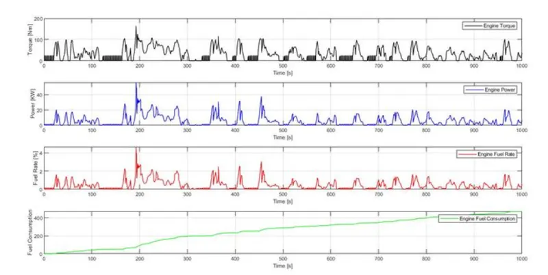
- Plot engine torque, engine power, fuel rate and fuel consumption using subplots.
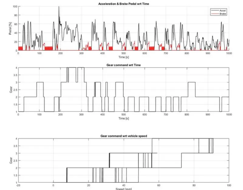
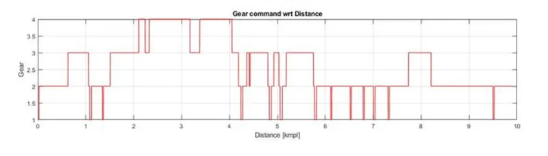
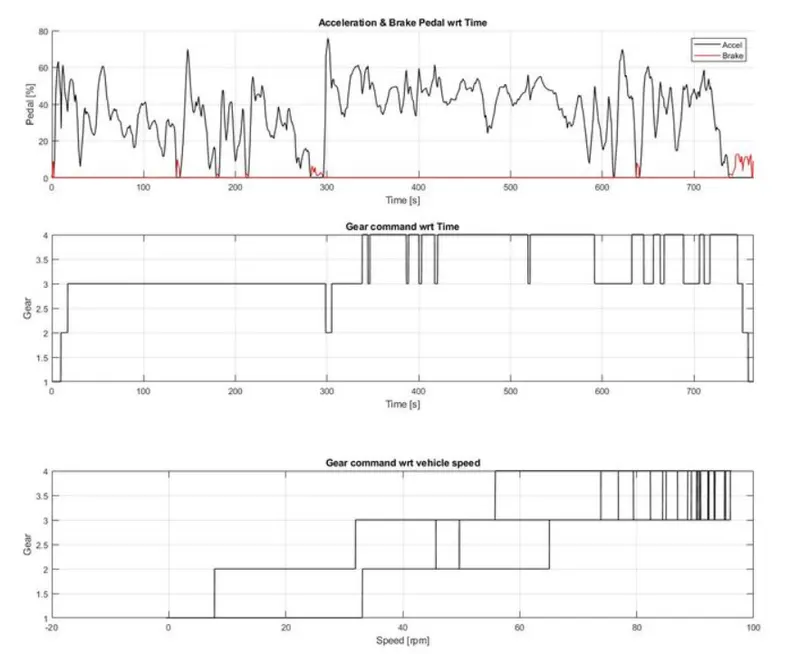
- Plot accelerator and brake pedal, gear command, vehicle desired and actual speed, vehicle distance using subplots.
- Plot the engine operating points on the engine fuel map.
- Plot motor speed, torque, motor input power using subplots.
- Plot pack voltage, current and SoC using subplots.
- Plot the motor operating points on the motor input power map, with the motor max motoring and generating torque curves.
- Write down appropriate brief comments on each of these plots, describing the vehicle behavior throughout the drive cycle.
- Generate the plots for both drive cycles
HEV:
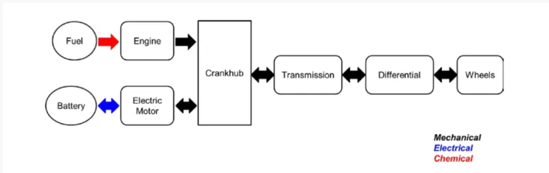
Hybrid electric vehicles (HEVs) are powered by an internal combustion engine in combination with one or more electric motors that use energy stored in batteries. HEVs combine the benefits of high fuel economy and low tailpipe emissions with the power and range of conventional vehicles.
In an HEV, the extra power provided by the electric motor may allow for a smaller combustion engine. The battery can also power auxiliary loads and reduce engine idling when the vehicle is stopped. Together, these features result in better fuel economy without sacrificing performance.
Model:
Matlab:
- A matlab code “Project2_InitFile.m” was created to load the variable to workspace.
- Honda Insight motor and battery are considered for this project. Data is taken from ADVISOR data base developed by NREL, USA. Data provided in the project files.
- The model developed has the capability to simulate the vehicle on different drive cycles like UDDS,HWFET,FTP,NEDC.

Code:
%% Initialization File
% Initialization file for loading the variables for the Conventional vehicle simulation model

%% Vehicle Parameters
M = 1500;       % Vehicle weight [kg]
Cr = 0.015;     % Rolling resistance coefficient
Rw = 0.35;      % Rolling radius [m]
Cd = 0.33;      % Drag coefficient
Af = 2;         % Frontal area [m2]
rhoa = 1.225;   % Air density [kg/m3]
Vwind = 0;      % Wind velocity [kmph]
g = 9.81;       % Gravitational acceleration [m/s2]
theta = 0;      % Slope [deg]
myu_road_tire = 1; % Coefficient of friction between tire - road interface

%% Powertrain Parameters
FDR = 3.73;                         % Final Drive Ratio / Diff Ratio
DiffEff = 0.99;                     % Differential efficiency (assumed independent of operating conditions)

NumGear = 4;                        % Number of gears in transmission
TransGear = [1:NumGear];            % Transmission Gears
TransRatio = [3.06, 1.62, 1, 0.7];  % Corresponding Transmission ratios
TransEff = 0.90;                    % Transmission efficiency (assumed independent of operating conditions)

TC_SR = [0, .5, .6, .7, .8, .87, .92, .94, .96, .97, 1];   % Torque Converter Speed Ratio (Matlab default) -> TurbSpd/PumpSpd
TC_TR = [2.232, 1.5462, 1.4058, 1.2746, 1.1528, 1.0732, 1.0192, 1, 1, 1, 1];   % Torque Converter Torque Ratio (Matlab default) -> TurbTrq/PumpTrq
TC_Cf = 1e-4 * [.72558, .66322, .63463, .59042, .51331, .4144, .29287, .22444, .12186, .04386, 0]; % Torque Converter Capacity Factor (Matlab default) -> PumpTrq/PumpSpd^2 [Nm/rpm^2]

load Vehicle_Data/Engine_data_1_9L_Saturn_95kW
load Vehicle_Data/Trans_Shift_map
load Vehicle_Data/EM_Honda_Insight_10kW
load Vehicle_Data/ESS_NiMH6


ESS_init_soc = 0.8;
ESS_soc_max = 0.9;
ESS_soc_min = 0.6;


%% Driver Parameters
Kp = 10;                    % P gain for driver PI model
Ki = 1;                     % I gain for driver PI model
Drive_Cycle_Select = 2;     % Drive cycle selection

% Drive cycle values in m/s

if Drive_Cycle_Select == 1
    load DriveCycles/UDDS;

elseif Drive_Cycle_Select == 2
    load DriveCycles/HWFET;

elseif Drive_Cycle_Select == 3
    load DriveCycles/FTP;

elseif Drive_Cycle_Select == 4
    load DriveCycles/US06;

elseif Drive_Cycle_Select == 5
    load DriveCycles/NEDC;

elseif Drive_Cycle_Select == 6
    load DriveCycles/WLTP;

end

time_end = cyc_time(end);
vel_end = cyc_vel(end);
The Simulink Model:
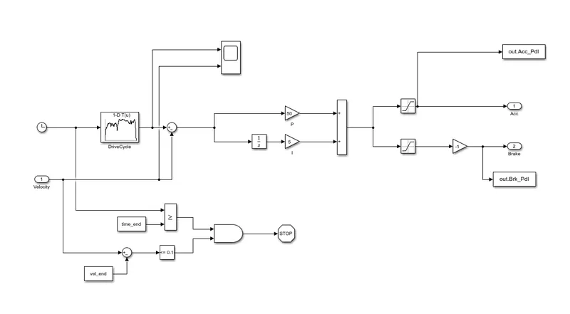
- Its modeled using a DRIVER BLOCK is a basic PI controller that generates accelerator and brake pedal outputs to match the desired and actual vehicle speeds.
- This accelerator and brake pedal data is generated using the drive cycle data in which is fed through look up table.
DRIVER BLOCK:
Controller Block:
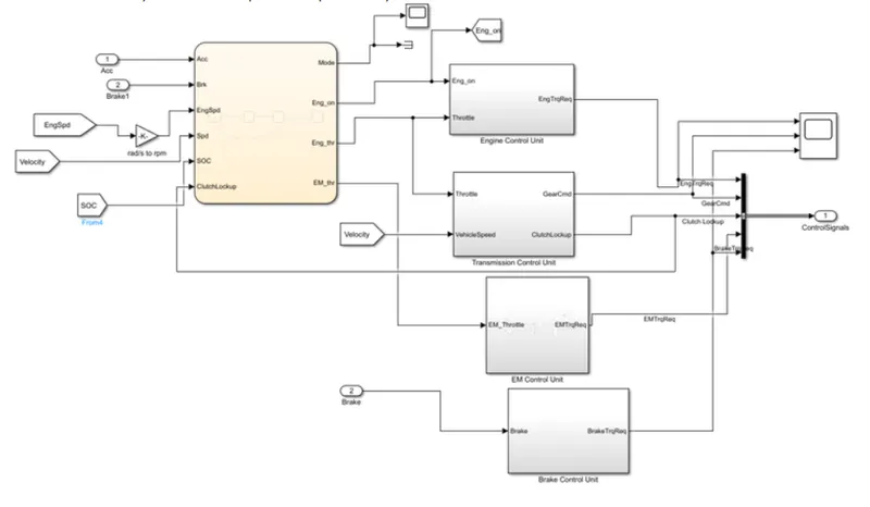
- The electric vehicle controller is the electronics package that operates between the batteries and the motor to control the electric vehicle's speed and acceleration much like a carburetor does in a gasoline-powered vehicle.
- Based on the driver inputs, it generates desired engine torque, desired transmission gear and desired brake torque and Em torque and the clutch lock up with the help of a supervisory controller.
State Flow Of Controller:
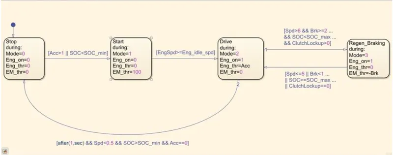
- In this we created four conditions as stop, start, drive and regenration braking. The initial block represent the stop
condition. In which the engine is off. The engine and motor throttle conditions are zero. Then the second block
represent start condition. In which the mode is 1 the electric motor throttle is only used to provide the required torque
and power to the vehicle. the engine is off and engine throttle conditionis zero. - The state 1 and state 2 are connected using the links i.e. it moves from state 1 to state 2 when acceleration is less than
‘one or SOC is less then the minimum SOC. - State 3 Represtents mode 2 ii.e. engine is on and the engine throttle is also having positive value from the driver but
the electric motor throttle is zero. It changes form state 2 to state 3 when engine speed is graeter than or equal to
engine idle speed. - state 4 represents regenrative braking which is model 3 In this state the engine is on but the engine throttle is having
no input from driver whereas the electric moto receives the negative power due to braking. - The inputs are given to chart is Acceleration, barke, engine speed, vehicle speed, SOC, and clutch lockup.
- The output we get from the chart is mode, engine condition, engine throttle condition, and electric motor throttle
condition.
Engine Controller Unit:
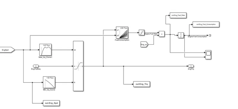
In this control model we use engine control unit in that give input,Engine speed through creating look up table,in that table we give input Maximum torque and map speed then also create 2nd block up trable in that input ct torque and map speed also give to ideal subtracts and multiplied.The engine speed also give an ideal control speed to intergate from this we meet output of the enigne required torque.
Electric Motor Block:
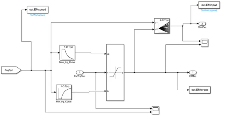
Shift logic unit:
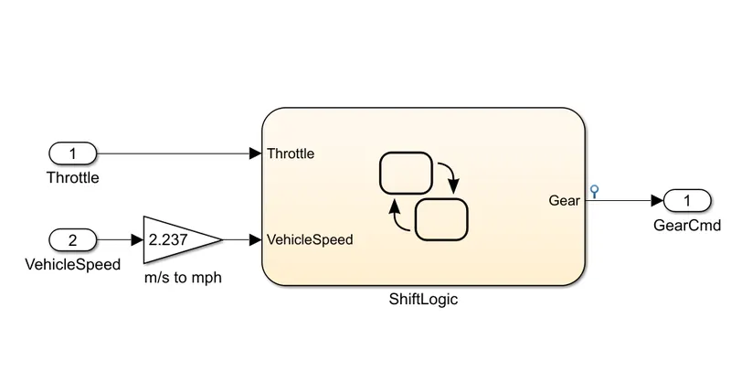
In this unit we create steadly flow variable state for controlling of gears of vehicle as in ascending and descending order with respect to time, speed,disteance and give input to tbis steady state is vehicle speed in m/s to mph.
Transmission Block:
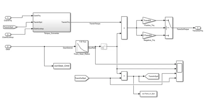
In these blocks we take engine torque, gear selector from controller from the transmission of the gear ratio.The ratioe is multiplied by transmission intput torque and then transmissin efficiency positive torque and negative torque gives transmission input speed. In this case torque converter connects the engine to transmission its part of transmission, basically engine dynamics and that is decoupled.
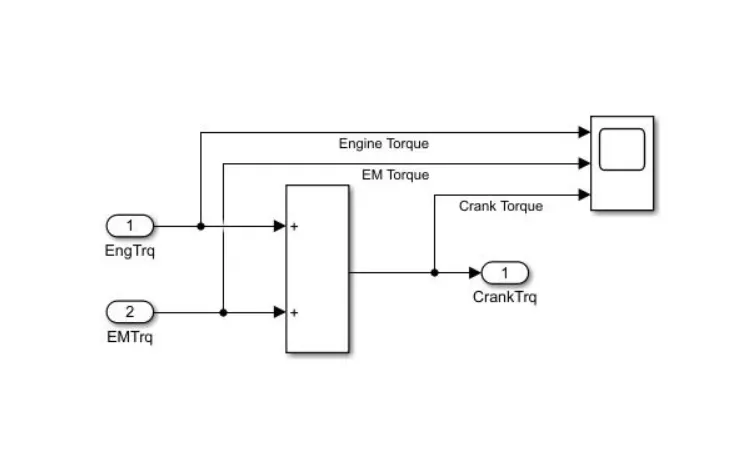
Crank hub:
Differential Block:
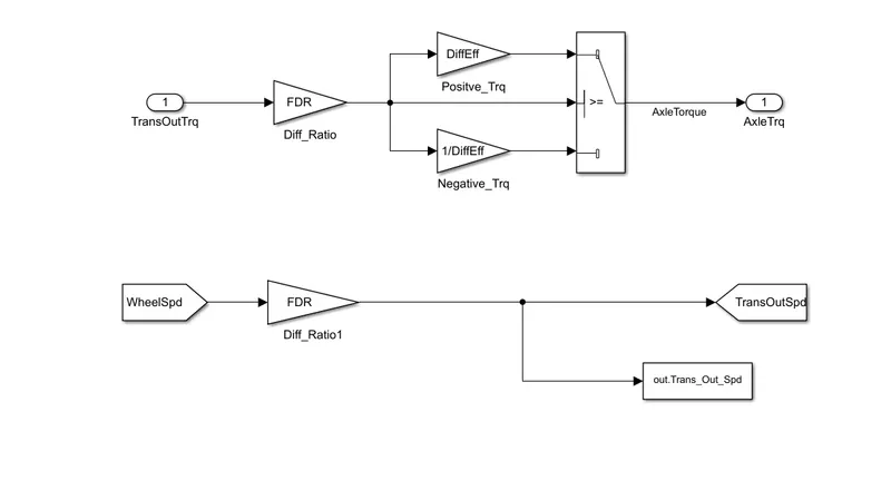
It takes input as the transmission output then iots goingto the differential ratio multiplied the output and input torque then meet axel torque.The axel torque is a lower than the transmission torque and differential ratio.
Wheel Block:
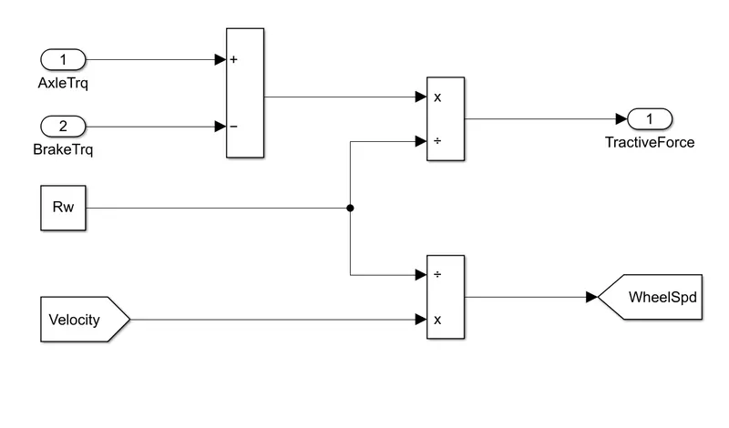
We take the axel torque from differential and brake torque from the controller.Its subtract and multiplied rolling radius anad velocity then we meet the tractive force from the axel and brake torque and the wheelspeed is meet using velocity.
Vehicle Dynamics Block:
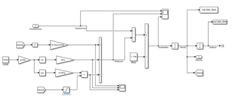
This takes tractive force and road load.It dictates vehicel speed based on the tractive force and road load.
Battery Modeling:
Storage system:
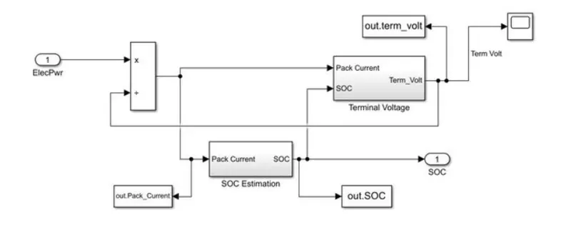
The input as poiwer then it multiply and give to pack current,then from the SOC estimation meet output SOC it gives terminal voltage as input and then meet terminal voltage as output.
Pack Current:
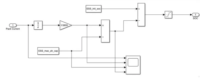 We integrate pack current and convert it from radian to amp then saturated and meet SOC.
Remaining Matlab Code:
%% Post-Processing File
%  File for post-processing the Conventional vehicle simulation model data

%% Renaming variables
Time = time_end;
Acc_Pdl = TC_SR;          % Accelerator pedal [%]
Brk_Pdl = TC_Cf;          % Brake pedal [%]
Gear_Cmd = TransGear;        % Transmission gear
Trans_In_Spd = TransEff*30/pi;  % Transmission input speed [rpm]
Trans_Out_Spd = Trans_In_Spd*30/pi;% Transmission output speed [rpm]
Eng_Trq = Eng_max_trq;          % Engine brake torque [Nm]
Eng_Spd = Eng_map_spd*30/pi;    % Engine speed [rpm]
Eng_Fuel_Consump = Eng_fuel_map;    % Engine fuel consumption [g]
Veh_Dist = vel_end/1000;   % Distance traveled by vehicle [km]
Veh_Spd = Eng_Spd*18/5;     % Vehicle speed [kmph]
wheel_speed = out.wheel_speed.data;
Eng_Fuel_rate = out.Eng_fuel_rate;
Veh_Desired_Speed = out.VEh_Desired_Spd;

Em_sped = out.EMspeed;
Wm_torq = out.EMtorque;
Em_PWR = out.EMinpwr;

Pack_current = out.packcurnt;
Pack_Voltg = out.packVoltg;
S_oc = out.s_o_c;


%% Data Analysis
Eng_Pwr = Eng_Spd.*pi/30.*Eng_Trq/1000;   % Engine brake power [kW]
rho_petrol = 0.7197;                    % Density of petrol [kg/L]
kmpl = Veh_Dist(end)/(Eng_Fuel_Consump(end)/1000/rho_petrol);  % Fuel economy [kmpl]

%% plotting Fuel Consumption vs Fuel Rate
Figure(1)
hold on
grid on
plot(Time, Eng_Fuel_Consump.Data,'linewidth',1,'color','black');
plot(Time, Eng_Fuel_rate.Data,'linewidth',1,'color,'red');

xlabel('Fuel Consumption')
ylabel('Fuel Rate')
xlim([0,Time(end)]);

%%plotting vehicle characteristics time trace engine, Transmission
figure(2)
hold on
grid on
plot(Time,Eng_Spd.Data,'linewidth',1,'color,'g');
plot(Time,Trans_In_Spd,'Linewidth',1,'Color,'black');
plot(Time,Trans_Out_Spd,'linewidth',1,'color,'red');
plot(Time,wheel_speed,'linewidth',1,'color',blue');

xlabel('Time[s]')
ylabel('speed[rpm]')
xlim([0,Time(end)]);
ylim([0,6000]);
legend('Transmission Input',Transmission Output','Wheel speed','Engine Speed');

%%plotting Vehicle Charateristics time trace engine torque, engine power, fuel rate and fuel consumption
figure(3)
subplot(2,2,1)
plot(Time,Eng_Trq.Data,'Linewidth','color','g')
xlabel('Time[s]')
ylabel('Torque[Nm]')
legend('Torque')

sub plot(2,2,2)
plot(Time,Eng_Pwr.Data,,'Linewidth','color','black')
xlabel('Time[s]')
ylabel('Power [kW]')
legend('Engine Power')

sub plot(2,2,3)
plot(Time,Eng_Fuel_rate.Data,'linewidth',1,'color','red')
xlabel(Time[s]')
ylabel('Fuel Rate[%]')
legend('Fuel Rate')

sub plot(2,2,4)
plot(Time,Eng_Fuel_Consump.Data,'linewidth',1,'color','blue')
xlabel(Time[s]')
ylabel('Fuel Consumption[kmpl]')
legend('Fuel Consumption')

%% Plotting vehicle characteristics time trace accelerator,and brake pedal,gear command, vehicle desired and actual speed
figure(4)
subplot(3,1,1)
hold on
grid on
plot(Time, TC_SR, 'linewidth', 1, 'Color', 'black');
plot(Time, TC_Cf, 'linewidth', 1, 'Color','blue ');
plot(time,wheel_speed,'linewidth',1,'color','red');
plot(Time,Trans_Out_Spd)
ylabel('Pedal [%]')
xlim([0, Time(end)]);
legend('Accel','Brake');

subplot(3,1,2)
hold on
grid on
plot(Time, Trans_In_Spd, 'linewidth', 1, 'Color', 'black');
plot(Time, Trans_Out_Spd, 'linewidth', 1, 'Color', 'red');
ylabel('Speed [rpm]')
xlim([0, Time(end)]);
ylim([0, 6000]);
legend('Trans Input','Trans Output');

subplot(3,1,3)
hold on
grid on
plot(Time, Gear_Cmd, 'linewidth', 1, 'Color', 'black');
xlim([0, Time(end)]);
xlabel('Time [s]');
ylabel('Gear');

%% Plotting engine operating points on engine fuel map
figure('Name','Engine Operating Points');
hold on
grid on
title('Engine Operating Points','fontsize',12);
p1=plot(Eng_map_spd*30/pi,Eng_max_trq,'linewidth',2,'color','r');
p2=line([Eng_map_spd(end)*30/pi Eng_map_spd(end)*30/pi],[0 Eng_max_trq(end)]);
set(p2,'linewidth',1,'linestyle','--','color','k');
p3=line([Eng_map_spd(1)*30/pi Eng_map_spd(1)*30/pi],[0 Eng_max_trq(1)]);
set(p3,'linewidth',1,'linestyle','--','color','k');
[c,h] = contour(Eng_map_spd'*30/pi,Eng_map_trq,Eng_fuel_map');
clabel(c,h);
xlabel('Engine Speed [rpm]');
ylabel('Engine Torque [Nm]');
title('Engine Fuel Consumption Map [g/s]');
%p4 = plot(Eng_Spd,Eng_Trq,'.','color','b');
legend([p1 p4],{'Max Curve','Operating Points'});
axis([Eng_map_spd(1)*30/pi Eng_map_spd(end)*30/pi 0 Eng_map_trq(end)]);


%%plotting motor speed, torque, motor input power
figure(7)
subplot(2,2,1)
plot(Time,EM_PWR.DATA,'Linewidth','color','g')
xlabel('Time[s]')
ylabel('Torque[Nm]')
legend('Torque')

sub plot(2,2,2)
plot(Time,EM_PWR.DATA,'Linewidth','color','black')
xlabel('Time[s]')
ylabel('Power[kW]')
legend('Engine Power')

sub plot(2,2,3)
plot(Time,Em_sped.Data,'linewidth',1,'color','red')
xlabel(Time[s]')
ylabel('Em speed')
legend('EM Speed')

%%plotting pack voltage, current and SOC
figure(8)
subplot(2,2,1)
plot(Time,Pack_currnt.Data,'Linewidth','color','g')
xlabel('Time[s]')
ylabel('Current')
legend('current')

sub plot(2,2,2)
plot(Time,Pack_voltg.Data,,'Linewidth','color','black')
xlabel('Time[s]')
ylabel('Voltage')
legend('Voltage')

sub plot(2,2,3)
plot(Time,S_oc.Data,'linewidth',1,'color','red')
xlabel(Time[s]')
ylabel('SOC')
legend('SOC')

%% Plotting EM operating points on EM map
figure('Name','Engine Operating Points');
hold on
grid on
title('Engine Operating Points','fontsize',12);
p1=plot(EM_map_spd*30/pi,EM_max_trq,'linewidth',2,'color','r');
p4=plot(EM_map_spd*30/pi,EM_max_trq,'linewidth',2,'color','black');
p2=line([EM_map_spd(end)*30/pi EM_map_spd(end)*30/pi],[0 EM_max_trq(end)]);
set(p2,'linewidth',1,'linestyle','--','color','k');
p3=line([EM_map_spd(1)*30/pi Eng_map_spd(1)*30/pi],[0 EM_max_trq(1)]);
set(p3,'linewidth',1,'linestyle','--','color','k');
[c,h] = contour(EM_map_spd'*30/pi,EM_map_trq,EM_fuel_map');
clabel(c,h);
xlabel('Engine Speed [rpm]');
ylabel('Engine Torque [Nm]');
title('EM input power');
legend([p1 p4 p3],{'Max Curve','Operating Points'});
axis([EM_map_spd(1)*30/pi EM_map_spd(end)*30/pi 0 EM_map_trq(end)]);
The above code is used to generate plots as given in the objectives.
Tabulate the fuel economy numbers (kmpl) for UDDS and HWFET cycle. Compare these numbers with the baseline numbers for conventional vehicle model from Project 1.
Answer:
Fuel Economy Number fo project 2
| S.NO | Drive Cycle | Fuel economy numbers (kmpl) |
| 1 | UDDS | 15.0773 |
| 2 | HWFET | 17.1613 |
From the abovre data we can conclude that HWFET is high compared to UDDS. Its because in the urban driving the vehicle encounters more traffic and its has to stop fo fever disatance and it consumes more fuel at the starting.
Comparing with fuel economy numbers of project1:
| S.NO | Drive Cycle | Fuel economy numbers (kmpl) |
| 1 | UDDS | 14.209 |
| 2 | HWFET | 16.503 |
The value is been high in project 2 than in project 2 because of the implementation of the Electric motor.
Plot the time trace for engine, transmission input, transmission output and wheel speed on one plot:
For UDDS Drive Cycle: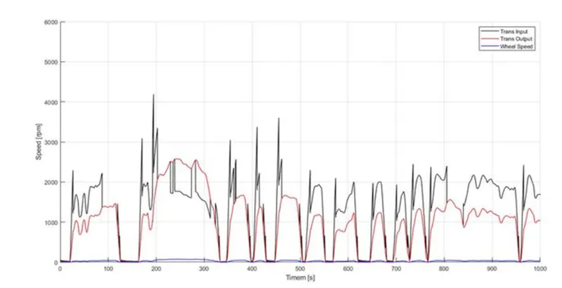
For HWFET Drive Cycle:
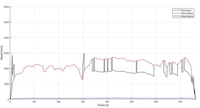
Plot the time trace for engine, transmission input, transmission output and wheel speed on one plot.
For UDDS Drive Cycle:
For HWFET Drive Cycle:
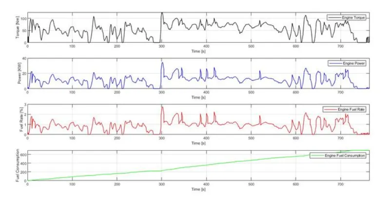
Plot engine torque, engine power, fuel rate and fuel consumption using subplots.
For UDDS Drive Cycle:
For HWFET Drive Cycle:
The Report link is shared:
https://docs.google.com/document/d/1jHiSNOlxL21UUQR2Cy3QKx3_Hky_-kyn/edit?usp=sharing&ouid=114352754031190187222&rtpof=true&sd=true