Project 2
1)solution:
Theory:
- The engine-to-wheel, rear-to-front, and cause-and-effect methods are other names for the forward modeling methodology. Calculation flows from engine to wheel in the same direction as positive power flow.
- This method is based on equations for vehicle dynamics, the behavior of individual powertrain parts, and their dynamic interplay.Moreover, a driver controller is necessary to guide the vehicle at a desired speed and
establish the commencement of the calculations. - The controller is set up to simulate how the driver will operate the brakes or the accelerator to match the intended speed,allowing for the study of driver behavior.
- The controller is utilized as a component of a feedback loop to calculate the amount of energy necessary to power the vehicle.
%%%%%%%%%%%%%%%%%%%%%%%%%%%%%%%%%%%%%%%%%%%%%%%%%%%%%%%%%%%%%%%%%%%%%
%% Skill-Lync -> Hybrid Drives Development
% Project 1 - Conventional Vehicle Model
% By - Ullekh Gambhira

% Description:

%% Initialization File
% Initialization file for loading the variables for the Conventional vehicle simulation model

%% Vehicle Parameters
M = 1500;       % Vehicle weight [kg]
Cr = 0.015;     % Rolling resistance coefficient
Rw = 0.35;      % Rolling radius [m]
Cd = 0.33;      % Drag coefficient
Af = 2;         % Frontal area [m2]
rhoa = 1.225;   % Air density [kg/m3]
Vwind = 0;      % Wind velocity [kmph]
g = 9.81;       % Gravitational acceleration [m/s2]
theta = 0;      % Slope [deg]
myu_road_tire = 1; % Coefficient of friction between tire - road interface
set_param('Project1_VehicleModel_FINAL','DataTypeOverride','Off');

%% Powertrain Parameters
FDR = 3.73;                         % Final Drive Ratio / Diff Ratio
DiffEff = 0.99;                     % Differential efficiency (assumed independent of operating conditions)

NumGear = 4;                        % Number of gears in transmission
TransGear = [1:NumGear];            % Transmission Gears
TransRatio = [3.06, 1.62, 1, 0.7];  % Corresponding Transmission ratios
TransEff = 0.90;                    % Transmission efficiency (assumed independent of operating conditions)

TC_SR = [0, .5, .6, .7, .8, .87, .92, .94, .96, .97, 1];   % Torque Converter Speed Ratio (Matlab default) -> TurbSpd/PumpSpd
TC_TR = [2.232, 1.5462, 1.4058, 1.2746, 1.1528, 1.0732, 1.0192, 1, 1, 1, 1];   % Torque Converter Torque Ratio (Matlab default) -> TurbTrq/PumpTrq
TC_Cf = 1e-4 * [.72558, .66322, .63463, .59042, .51331, .4144, .29287, .22444, .12186, .04386, 0]; % Torque Converter Capacity Factor (Matlab default) -> PumpTrq/PumpSpd^2 [Nm/rpm^2]

load Vehicle_Data/Engine_data_1_9L_Saturn_95kW
load Vehicle_Data/Trans_Shift_map

%% Driver Parameters
Kp = 10;                    % P gain for driver PI model
Ki = 1;                     % I gain for driver PI model
Drive_Cycle_Select = 1;     % Drive cycle selection

% Drive cycle values in m/s

if Drive_Cycle_Select == 1
    load DriveCycles/UDDS;

elseif Drive_Cycle_Select == 2
    load DriveCycles/HWFET;

elseif Drive_Cycle_Select == 3
    load DriveCycles/FTP;

elseif Drive_Cycle_Select == 4
    load DriveCycles/US06;

elseif Drive_Cycle_Select == 5
    load DriveCycles/NEDC;

elseif Drive_Cycle_Select == 6
    load DriveCycles/WLTP;

end

time_end = cyc_time(end);
vel_end = cyc_vel(end);
Simulink Model:
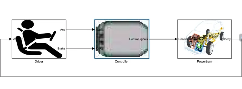
- The driver model, control model, and powertrain block are the three basic sub-blocks used to form the convection model in Simulink.
- The controller block sends control signals for engine torque, gear shifting, and brake torque to the Powertrain model while the driver block receives feedback on the actual
- vehicle speed and supplies the controller block with the necessary acceleration or braking output.
Driver Model:
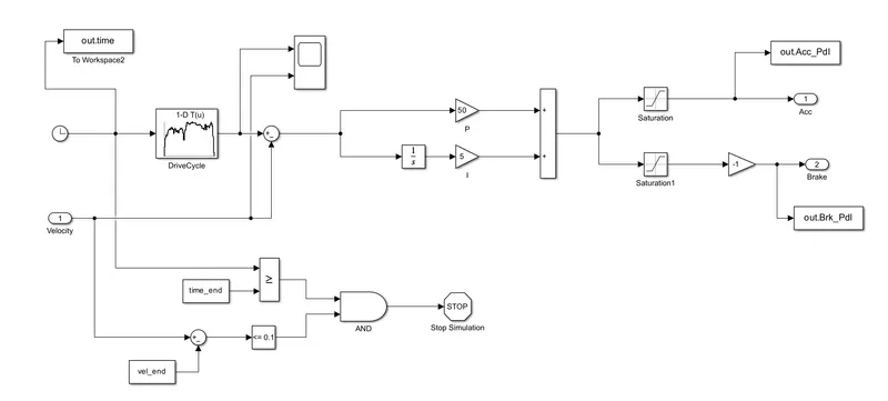
- The transmission model, which depicts the drive train, receives all control signals again.
- A fundamental PI controller called Driver Model produces outputs from the accelerator and brake pedals that are matched to the desired and actual vehicle speeds.By giving the controller output for the accelerator and brake pedals, the PI controller manages the discrepancy between the needed driving cycle and the actual vehicle speed
Controller Block:
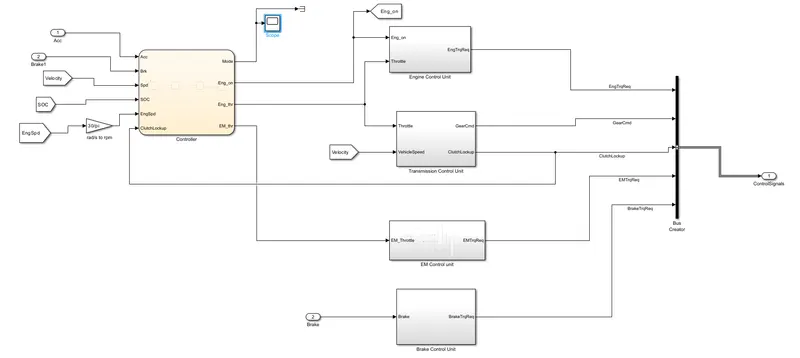
- The vehicle's "Controller block," which stands in for the electronic control modules,is its brain. It produces the required engine torque, desired motor torque, desired transmission gear, and desired brake torque based on the driver's inputs. These inputs are supplied to the "Powertrain" block, which symbolizes the vehicle's drivetrain
- The supervisory control unit, which selects the operation modes (start/stop, cruise, or regeneration braking mode. The engine drive and the motor drive are adjusted for each mode.
- The driver unit's input for the accelerator and brake pedals, the engine's actual speed,the vehicle's actual speed, the SOC status, and the clutch lockup state are the inputs for The state flow charts.
- Moreover, the Mode, Engine On/Off Request, Engine Input Throttle, and Electric Motor Input Throttle are the State flow Outputs to the Individual Controllers.
- The controller is made up of an electric motor control unit, a brake control unit, an engine control unit, and a transmission control unit.
Controller subsystem:
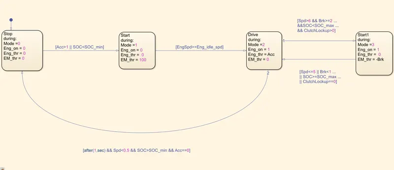
- The driver unit's input for the accelerator and brake pedals, the engine's actual speed,the vehicle's actual speed, the SOC status, and the clutch lockup state are the inputs for the state flow charts. Moreover, the Mode,Engine On/Off Request, Engine Input
- Throttle, and Electric Motor Input Throttle are the State flow Outputs to the Individual Controllers.
- The controller is made up of an electric motor control unit, a brake control unit, an engine control unit, and a transmission control unit.
- The transmission model, which depicts the drive train, receives all control signals again.
Engine Control Unit:
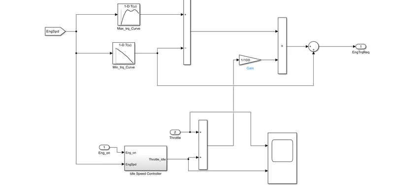
In the engine control unit there is two 1d lookup tables are added and fed into the throttle input also fed into product block and idle torque converter is used here control the throttle input.
Idle Speed Controller:
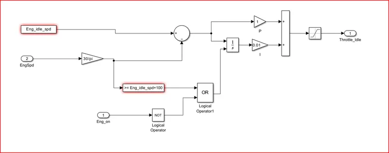
The idle speed controller block is a component of an engine control system that regulates the engine's idle speed. It operates by adjusting the airflow to the engine's throttle body, either by controlling the throttle plate or bypassing air around it. The controller typically receives input from various sensors, such as the engine temperature and throttle position sensors, to determine the appropriate idle speed. If the idle speed drops too low or rises too high, the controller adjusts the airflow accordingly to maintain a stable idle. Proper functioning of the idle speed controller is crucial for smooth engine operation and can also affect emissions and fuel economy.
Electric machine Control Unit:
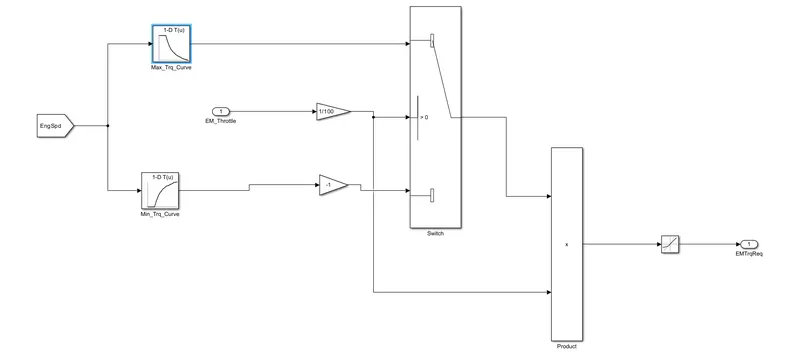
Drive Motor Unit Give the Electric Motor the necessary torque command by comparing its speed to the maximum torque curve and maximum torque generation curves in the lookup table. In order to compare the lookup tables and determine the torque input needed for the E-Motor, the EM throttle input is employed for this block.
Transmission Control Unit:
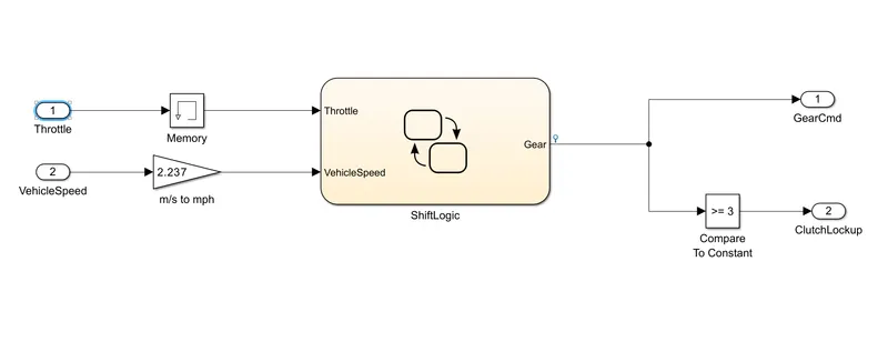
For this block the transmission control logic unit we are adding memry block to save the driver input feed. we are getting input in the form of m/s need to convert in mph. there is a compare to constant block from thre out of gear model for the clutchlockup output.
Transmission Control unit Shift Logic:
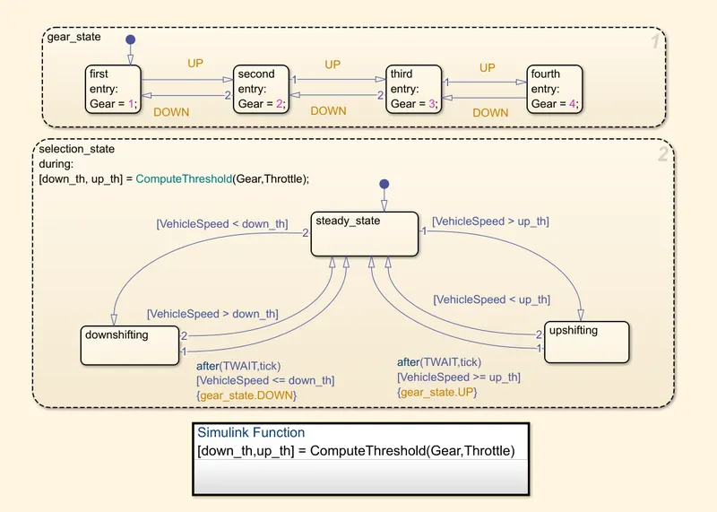
here we using this block for gear selection state we are getting output and gear changing according to the driver input comapre to the threshold value with gear and throttle.
Brake Control Unit:
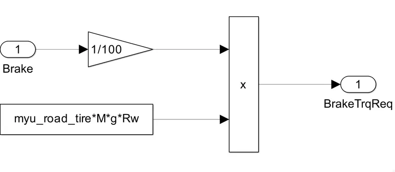
Brake controller generates the necessary brake torque in accordance with the input fromthe brake pedal, then transmit that torque to the wheel block in the transmission model.
powertrain Model:
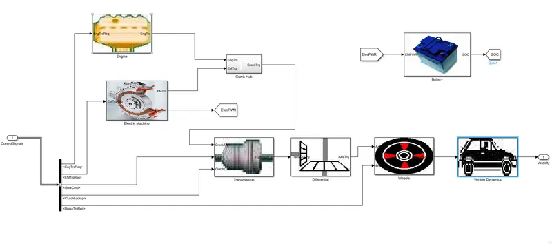
The Powertrain model consist of Engine,transmission,Gearbox,Differential,wheel,vehicle dynamics for the conventional IC engine model for the Hybrid drive model ther Electric motor and battery is added to thr powertain block .Engine output is fed into the input for the electric motor from the motor we are gettiing Torque And electric power as the output. The Output from thre electric motor is given to the Battery input.
Engine Unit:
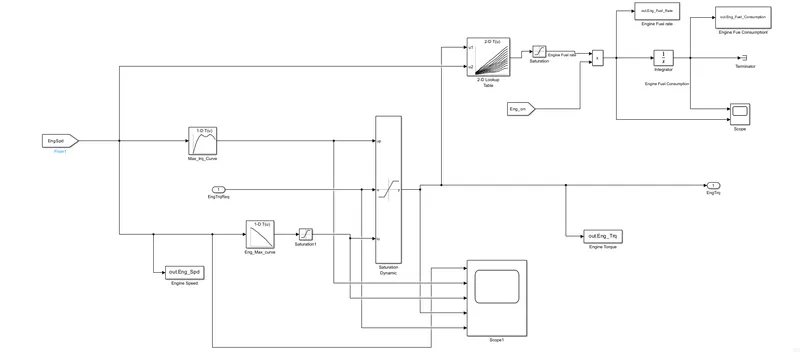
In the Engine We are giving the input as the Engine Speed and we are using the saturation dynamic and saturation block to limit the Engine Speed also we are using the 1d lookup tables for the extrapolation values we are getting the output as the fuel rate and the fuel consumption.
Electric machine:
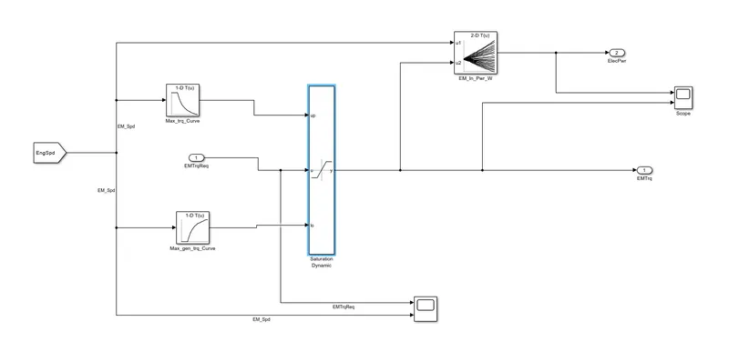
The clutch lock up condition of the torque converter determines the pump and turbine torque, and the combination provides the necessary transmission torque.
Transmission Unit:
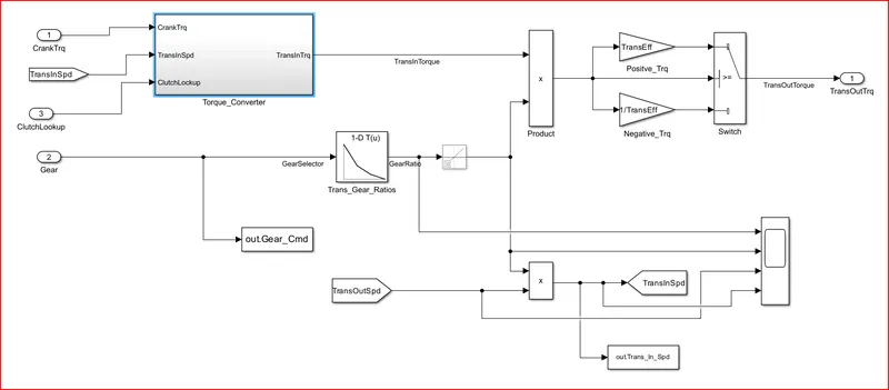
In the transmission unit there is newly added clutchlockup into thius torque converter block and we get the output as the Trans torque from torque conveter.There is 1D lookup table for the transgearratio and find the extra polated values also.
Differential unit:
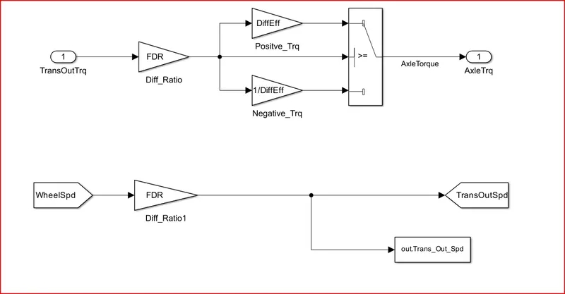
In the Differential Unit we are feeding Transout ytorque and the Wheel speed as a input and Tranouttorque is multiplied with final drive ratio value to get the Positive and negative torque values by using the Switch block we are getting Axle Torque.
Wheel Unit:
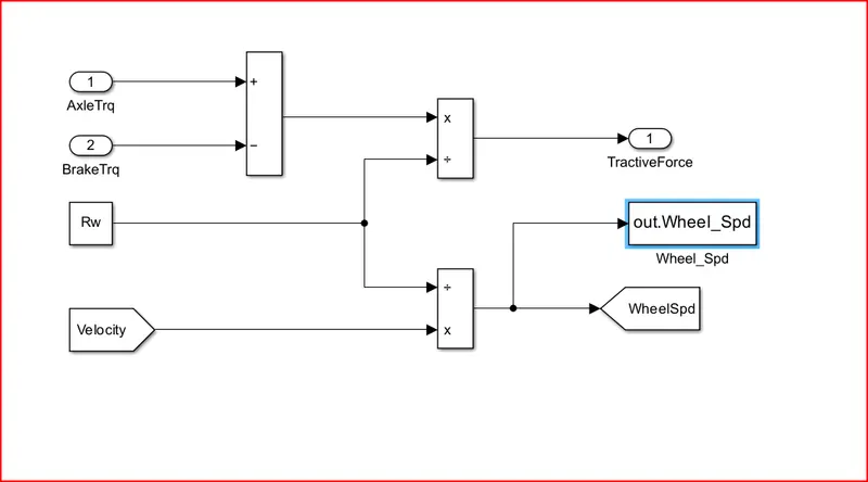
To calculate the tractive force, the axle torque from the control model is subtracted from the brake torque, which is then divided by the rolling radius.The vehicle velocity is used to calculate the Wheel speed, which is then saved in the workspace
Vehicle Dynamics:
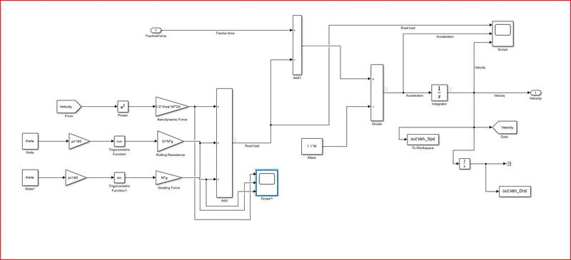
in this block There is road load and three forces acting on the vehicle that is Aerodynamic force,rolling Resistance and Tractive force which will be added to form the road load the road will feed into the mass block and we get the Actual Vehicle Speed and vehcle distance runnning on the Vehicle shown in that block.
Matlab Graphs:
Project 2- Processing File
%%%%%%%%%%%%%%%%%%%%%%%%%%%%%%%%%%%%%%%%%%%%%%%%%%%%%%%%%%%%%%%%%%%%%
%% Skill-Lync -> Hybrid Drives Development
% Project 1 - Conventional Vehicle Model
% By - Ullekh Gambhira

% Description:
% The following file is to used with the Initialization file and Simulink
% results for post-processing of the data.
% The file is incomplete, has some examples of how the data is imported
% into a readable format, data analysis, and plotting examples.
% Based on the project task, use commands in a similar format as given
% below to analyze the data and generate the required plots.
% You can change variable names if desired

%% Post-Processing File
%  File for post-processing the Conventional vehicle simulation model data

%% Renaming variables
Time = out.time;
Acc_Pdl = out. Acc_Pdl;          % Accelerator pedal [%]
Brk_Pdl = out. Brk_Pdl;          % Brake pedal [%]
Gear_Cmd = out. Gear_Cmd;        % Transmission gear
Trans_In_Spd = out. Trans_In_Spd*30/pi;  % Transmission input speed [rpm]
Trans_Out_Spd = out. Trans_Out_Spd*30/pi;% Transmission output speed [rpm]
Eng_Trq = out. Eng_Trq;          % Engine brake torque [Nm]
Eng_Spd = out. Eng_Spd*30/pi;    % Engine speed [rpm]
Eng_Fuel_Consump = out. Eng_Fuel_Consumption;    % Engine fuel consumption [g]
Eng_Fuel_rate=out.Eng_Fuel_Rate;          % engine Fuel rate in [g/s]
Veh_Dist = out. Veh_Dist/1000;   % Distance traveled by vehicle [km]
Veh_Spd = out. Veh_Spd*18/5;     % Vehicle speed [kmph]
Wheel_Spd = out. Wheel_Spd;
SOC=out.soc;
V_term=out.term_volt;
I_pack=out.Current;
EM_power=out.EM_PWR;
EM_torque=out.EM_Trq;
EM_Spd=out.EM_Spd;
Actual_Speed=out.Actual_Spd;
Desired_Speed=out.Desire_Spd;

%% Data Analysis
Eng_Pwr = Eng_Spd.*pi/3.*Eng_Trq/1000; % Engine brake power [kW]
rho_petrol = 0.7197;                    % Density of petrol [kg/L]
kmpl = Veh_Dist(end)/(Eng_Fuel_Consump(end)/1000/rho_petrol);    % Fuel economy [kmpl]
fprintf('nFuel Economy = %2.2fKmpl',kmpl);

%% Plotting engine operating points on engine fuel map
figure('Name','Engine Operating Points');
hold on
grid on
title('Engine Operating Points','fontsize',12);
p1=plot(Eng_map_spd*30/pi,Eng_max_trq,'linewidth',2,'color','r');
p2=line([Eng_map_spd(end)*30/pi Eng_map_spd(end)*30/pi],[0 Eng_max_trq(end)]);
set(p2,'linewidth',1,'linestyle','--','color','k');
p3=line([Eng_map_spd(1)*30/pi Eng_map_spd(1)*30/pi],[0 Eng_max_trq(1)]);
set(p3,'linewidth',1,'linestyle','--','color','k');
[c,h] = contour(Eng_map_spd'*30/pi,Eng_map_trq,Eng_fuel_map');
clabel(c,h);
xlabel('Engine Speed [rpm]');
ylabel('Engine Torque [Nm]');
title('Engine Fuel Consumption Map [g/s]');
%p4 = plot(Eng_Spd,Eng_Trq,'.','color','k');
legend([p1 p3],{'Max Curve','Operating Points'});
axis([Eng_map_spd(1)*30/pi Eng_map_spd(end)*30/pi 0 Eng_map_trq(end)]);


%% Plot pack voltage, current and SoC using subplots.

figure(3)
subplot(311)
plot(SOC,'k');
title('State Of Charge vs Time');
ylabel('State Of Charge (%)');
legend('SOC');
xlim([0 time(end)])

subplot(312)
plot(V_term,'g');
title('Terminal Voltage vs Time');
ylabel('Terminal Voltage (V)');
legend('Terminal Voltage');
xlim([0 Time(end)])

subplot(313)
plot(I_pack,'m');
title('Pack Current vs Time');
ylabel('pack current (A)');
legend('Pack Current');
xlim([0 Time(end)])

%% Plot accelerator and brake pedal, gear command, vehicle desired and actual speed, vehicle distance using subplots.

figure();
subplot(511)
plot(Time,Acc_Pdl,'r',Time,Brk_Pdl,'c');
ylabel('Pedal [%]');
xlabel('Time (Sec)');
title('Accl Pdl vs Brk Pdl vs Time');
xlim([0 Time(end)])
legend('Acc Pedal','Brake Pedal',Location='best');

subplot(512)
plot(Time,Gear_Cmd,'k');
ylabel('Gear');
xlabel('Time (Sec)');
title('Gear Cmd vs Time');
legend('gear Command',Location='best');
xlim([0 Time(end)])

 subplot(513)
 plot(Time,Veh_Dist,'b');
 ylabel('Distance [Km]');
 xlabel('Time (Sec)')
  title('Vehicle Dist vs Time');
 legend('Vehicle Distance',Location='best');
 xlim([0 Time(end)])

 subplot(514)
 plot(Actual_Speed,'r','Linewidth',1,'Color','c');
ylabel('Speed [Kmph]');
xlim([0 Time(end)])
title('Actual Speed vs Time');
legend('Actual Speed',Location='best');

 subplot(515)
plot(Desired_Speed,'m');
 ylabel('Speed [Kmph]');
 xlim([0 Time(end)]);
 title('Desired Speed vs Time')
 legend('Desired Speed',Location='best');

%% Plot engine torque, engine power, fuel rate and fuel consumption using subplots.
figure(6)
subplot(411)
plot(Time,Eng_Trq,'LineWidth',1,'Color','m');
legend('Engine Torque');
ylabel('Engine Torque [Nm]');
title('Engine Torque vs Time');
xlim([0 Time(end)]);

subplot(412)
plot(Time,Eng_Pwr,'LineWidth',1,'Color','b','LineStyle','--');
legend('Engine Power');
ylabel('Power in KW');
title('Engine Power vs Time');
xlim([0 Time(end)]);

subplot(413)
plot(Time,Eng_Fuel_Consump,'LineWidth',1,'Color','r','LineStyle','-');
legend('Fuel Consumption');
ylabel('Fuel Consumption [g]');
title('Fuel Consumption vs Time');
xlim([0 Time(end)]);

subplot(414)
plot(Time,Eng_Fuel_rate,'LineWidth',1,'Color','k');
legend('Engine Power');
title('Fuel Rate vs Time');
ylabel('Power in KW');
xlabel('Time (Sec)');
xlim([0 Time(end)]);

%%  Plot the time trace for engine, transmission input, transmission output and wheel speed on one plot.
figure()
subplot(311)
plot(Time,Wheel_Spd,'LineWidth',1,'Color','r');
xlabel('Time (Sec)');
ylabel('Speed [rpm]');
title('Wheel Speed vs Time');
legend('Wheel Speed');
xlim([0 Time(end)]);

subplot(312)
plot(Time,Trans_In_Spd,'LineWidth',1,'Color','b');
xlabel('Time (Sec)');
ylabel('Speed [rpm]');
title('TransIn SpeedSpeed vs Time');
legend('Transin Spd');
xlim([0 Time(end)]);

subplot(313)
plot(Time,Trans_Out_Spd,'LineWidth',1,'Color','k','LineStyle','--');
xlabel('Time (Sec)');
ylabel('Speed [rpm]');
title('Transout Speed vs Time');
legend('Transout Spd');
xlim([0 Time(end)]);

%% Plot motor speed, torque, motor input power using subplots.
figure()
subplot(311)
plot(Time,EM_Spd,'LineWidth',1,'Color','r');
ylabel('Speed [rpm]');
xlabel('Time (Sec)');
legend('EM Spd');
title('Elecric Motor vs Time');
xlim([0 Time(end)])

subplot(312)
plot(Time,EM_power,'LineWidth',1,'Color','k');
ylabel('Power [KW]');
xlabel('Time (Sec)');
legend('EM Power');
title('Elecric Power vs Time');
xlim([0 Time(end)])

subplot(313)
plot(Time,EM_torque,'LineWidth',1,'Color','b');
ylabel('Torque [Nm]');
xlabel('Time (Sec)');
legend('EM Torque');
title('Elecric Torque vs Time');
xlim([0 Time(end)])

%%  Plot the motor operating points on the motor input power map, with the motor max motoring and generating torque curves.

figure ('Name','Motor Operating Points');
hold on
grid on
title('Engine Operating Points','FontSize',12);
p1=plot(EM_map_spd*30/pi,EM_max_trq,'LineWidth',2,'Color','r');

p4=plot(EM_map_spd*30/pi,EM_max_gen_trq,'LineWidth',2,'Color','k');

p2=plot([EM_map_spd(end)*30/pi EM_map_spd(end)*30/pi],[0 EM_max_trq(end)]);
set(p2,'LineWidth',1,'Color','b','LineStyle','-');

p3=line([EM_map_spd(1)*30/pi EM_map_spd(1)],[0 EM_max_trq(1)]);
set(p3,'LineWidth',1,'LineStyle','--','Color','m');
[c,h]= contour(EM_map_spd*30/pi,EM_map_trq,EM_inpwr_map');
clabel(c,h);
xlabel('EM Speed [rpm]');
ylabel('EM Torque [Nm]');
title('EM Input Power');
legend([p1 p4 p3],{'Max Curve','Regen Curve','Operating Points'});
Tabulate the fuel economy numbers (kmpl) for UDDS and HWFET cycle. Compare these numbers with the baseline numbers for conventional vehicle model from Project 1
| Fuel Economy [Kmpl] | Project 1 | P1 Model |
| UDDS | 24.82 | 26.11 |
| HWFET | 37.81 | 36.17 |
Conclusion: From the tabulated value we get HWFET gives more fuel economy
UDDS Cycle:
drive Cycle:
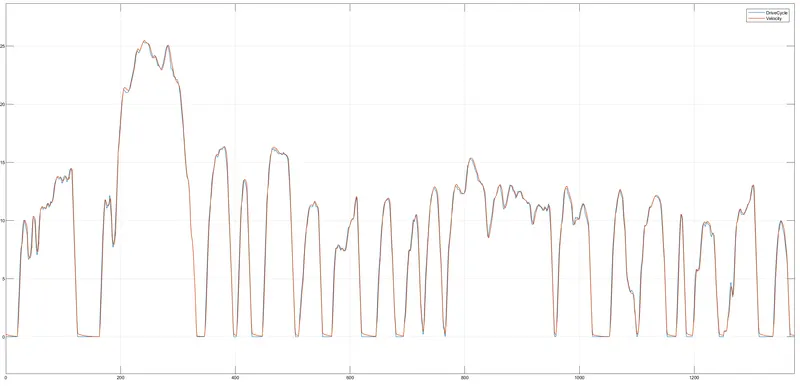
The UDDS drive cycle graph is a standardized test used to evaluate the emissions and fuel economy of vehicles under real-world driving conditions. The UDDS drive cycle graph shows the speed and acceleration of a vehicle over a period of time, and is designed to simulate typical urban driving conditions. The UDDS drive cycle graph is an important tool for assessing the environmental impact of vehicles.
accelerator and brake pedal, gear command, vehicle desired and actual speed, vehicle distance
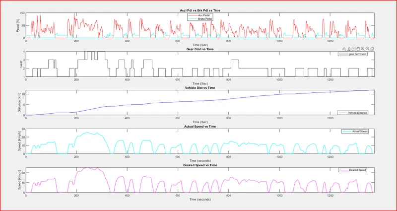
Here we are comapring the Accelerator pedal,Brake pedal,Actual Speed vs Desired Speed And Vehicle Distance and Gear command. Actual Speed is Vehicle Speed and Desired Speed for predetermined Speed.Vehicle distance increases when time increases.
pack voltage, current and SoC in UDDS
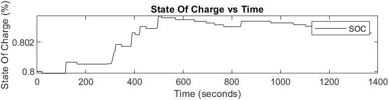
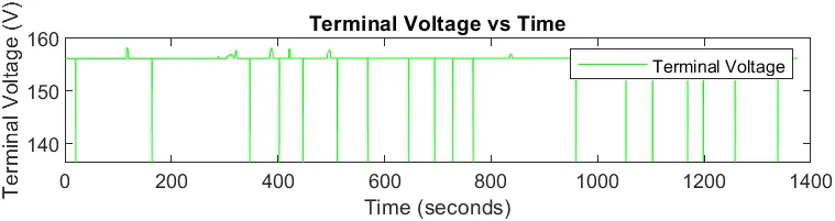
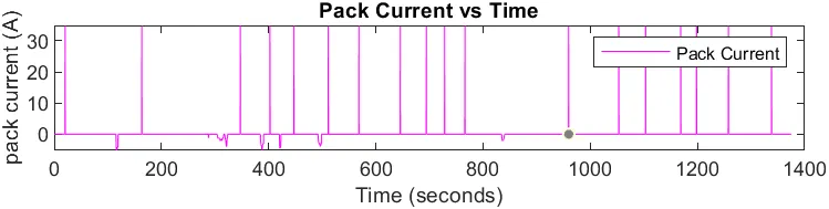
This block pack current and terminal voltage is opposite to each other and fluctuate more with regarding the time increases. we plot the graph against the SOC,Pack current and Terminal Voltage vs time the terinal voltage is connected as closed loop system, to compare the SOC value the Soc value rage from 60 to 90 percentage.
The engine operating points on the engine fuel map for UDDS
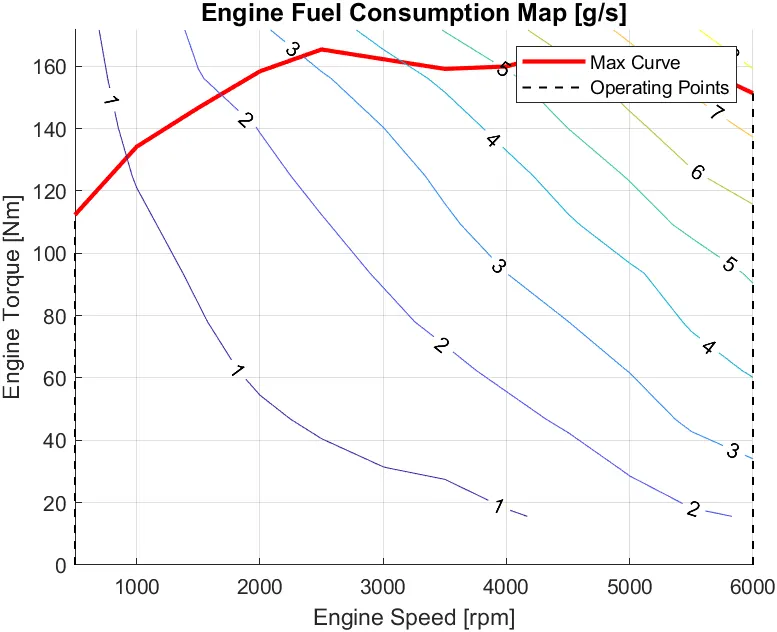
This block is created using contour command and we plot only the p1 and p3 line sother lines are set as fixed. here operating situate at the maximum speed and maximum torque is increasing with the Increase of Speed.
The engine torque, engine power, fuel rate and fuel consumption using subplots (UDDS)
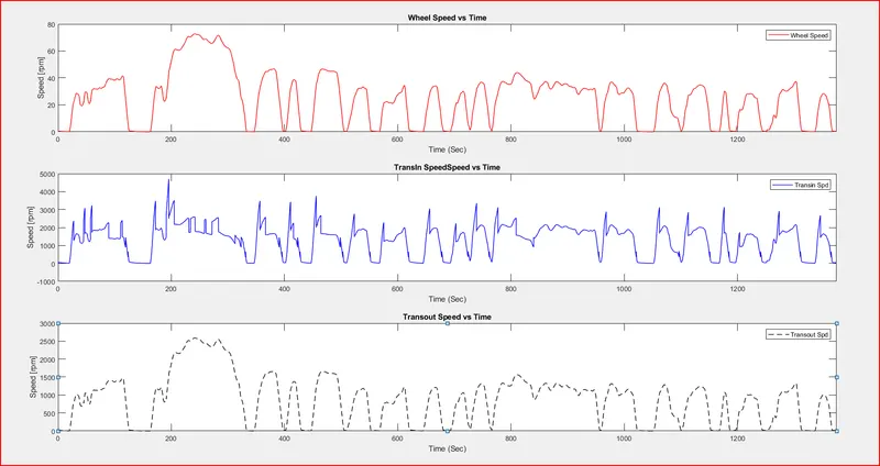
In this block we check the wheel speed with the Transmission input speed and Transmission output speed.Here we are seeing the Transout speed is similar to the wheel speed, Transmissiion input speed chages according to the input we are given.
The time trace for engine, transmission input, transmission output and wheel speed on one plot
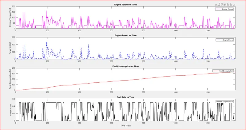
The block we need to compare the Engine power,Engine Torque, Fuel cosumption and Fuel Flow rate.the fuel consumption increases with the time increases.The engine power is uptained from engine Speed.
Electric motor Speed,Electric Torque and Electric Power
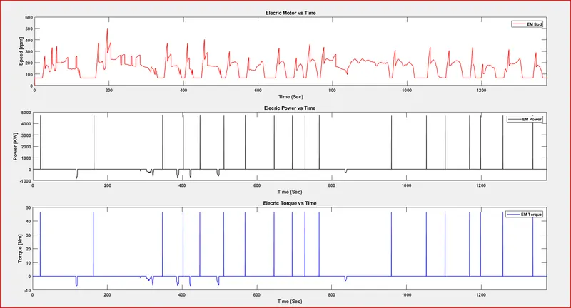
electric motor graph is created by using the Electric power we are getting from the Engine Speed we are taken as the Electric Motor Speed and Electric power and Elctric Torque iscreated by using the Workspace block and time running for 1260 seconds.
Plot the motor operating points on the motor input power map, with the motor max motoring and generating torque curves.
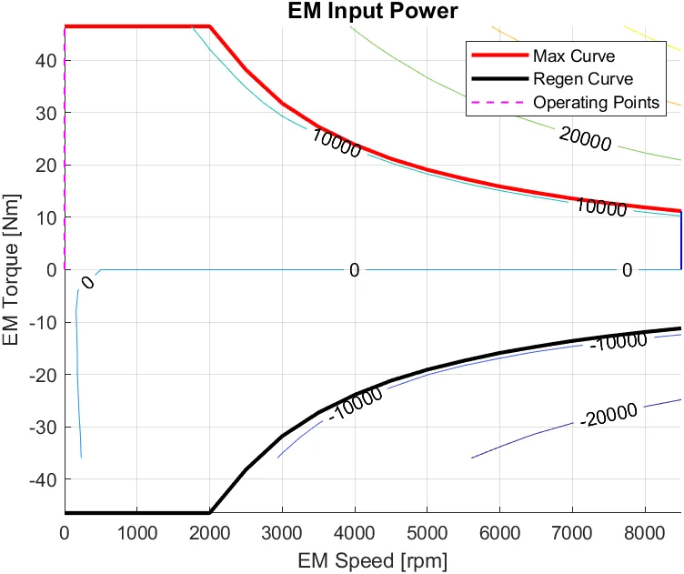
from this graph we are comapring first and last value of the electric motor input power curve and fit the operating into this graph. plotthe graph engine Speed vs Engine max torque.
HWFET Cycle:
Drive Cycle:
The Highway Fuel Economy Test (HWFET or HFET) cycle is a chassis dynamometer driving schedule developed by the US EPA for the determination of fuel economy of light duty vehicles .The HWFET is used to determine the highway fuel economy rating, while the city rating is based on the FTP-75 test and the otalduration for this cycle is 765 seconds.
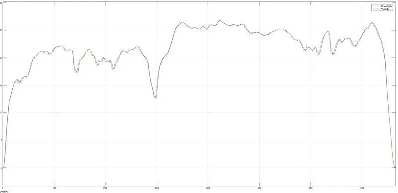
The HWFET drive cycle graph shows the time-speed data points of the cycle, which is a chassis dynamometer driving schedule developed by the US EPA for the determination of fuel economy of light-duty vehicles.The graph shows the speed of the vehicle over time, with the goal of achieving a steady-state speed of 48.3 mph (77.7 km/h) for the majority of the cycle.The cycle has a duration of 765 seconds and covers a total distance of 10.26 miles (16.45 km).The HWFET is used to determine the highway fuel economy rating of light-duty vehicles in the US.
Accelerator and brake pedal, gear command, vehicle desired and actual speed, vehicle distance using subplots
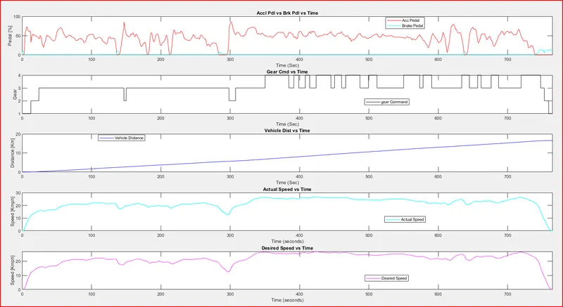
Here we are comapring the Accelerator pedal,Brake pedal,Actual Speed vs Desired Speed And Vehicle Distance and Gear command. Actual Speed is Vehicle Speed and Desired Speed for predetermined Speed.Vehicle distance increases when time increases.
The time trace for engine, transmission input, transmission output and wheel speed on one plot
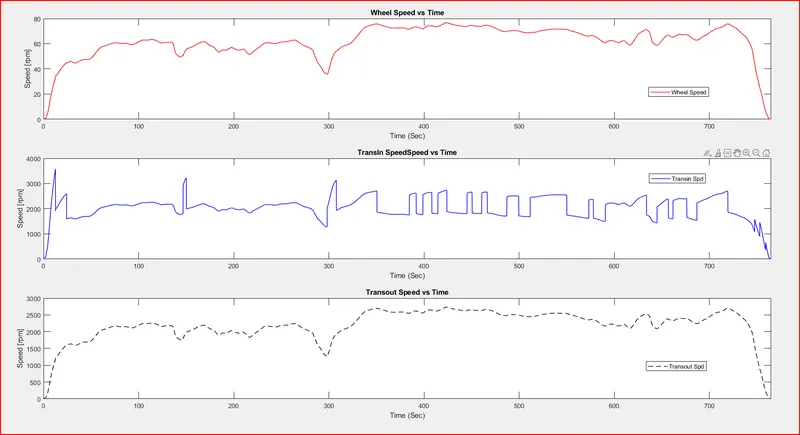
In this block we check the wheel speed with the Transmission input speed and Transmission output speed.Here we are seeing the Transout speed is similar to the wheel speed, Transmissiion input speed chages according to the input we are given.
Engine torque, engine power, fuel rate and fuel consumption using subplots
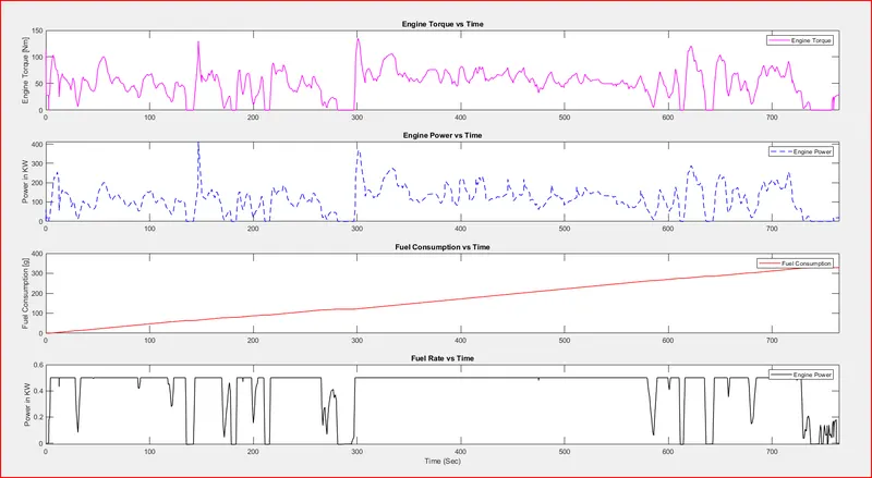
The block we need to compare the Engine power,Engine Torque, Fuel cosumption and Fuel Flow rate.the fuel consumption increases with the time increases.The engine power is uptained from engine Speed.
The engine operating points on the engine fuel map
This block is created using contour command and we plot only the p1 and p3 line sother lines are set as fixed. here operating situate at the maximum speed and maximum torque is increasing with the Increase of Speed.
Pack voltage, current and SoC using subplots
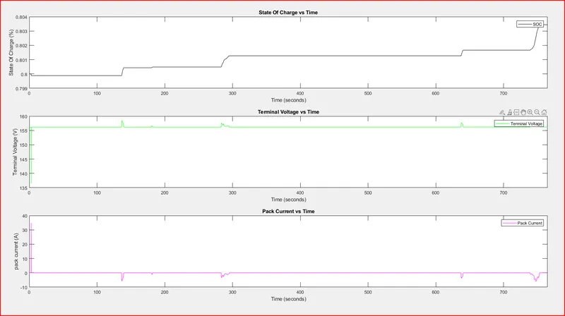
This block is taken from the week 9 challenge we plot the graph against the SOC,Pack current and Terminal Voltage vs time the terinal voltage is connected as closed loop system, to compare the SOC value the Soc value rage from 60 to 90 percentage.
Electric Motor speed, torque, motor input power using subplots
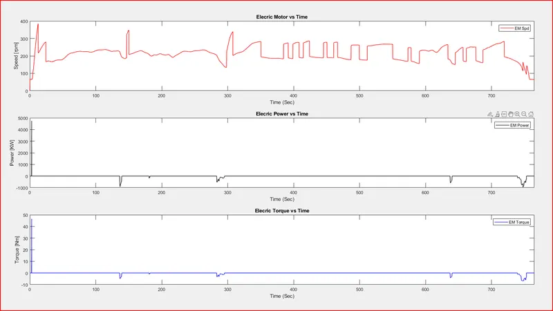
electric motor graph is created by using the Electric power we are getting from the Engine Speed we are taken as the Electric Motor Speed and Electric power and Elctric Torque iscreated by using the Workspace block and time running for 765 seconds.
The motor operating points on the motor input power map, with the motor max motoring and generating torque curves
from this graph we are comapring first and last value of the electric motor input power curve and fit the operating into this graph. plotthe graph engine Speed vs Engine max torque.
Conclusion:
The UDDS and HWFET cycle charts have been created for the forward energy-based fuel consumption model of a hybrid electric vehicle and the fuel economy number for each driving cycle was compared with the a conventional vehicle subjected to the same driving conditions. The main observations were as follows:
As the engine's power loss is reduced, fuel economy number enhances. Regenerative breaking can restore negative energy.The fuel economy number is higher for HWFET drive cycle compared to UDDS, due to less power loss. Even though, the lost power will be recaptured by regenerative braking, and thus increases battery SOC. Because there is more brake pedal engagement and idle time during the UDDS drive cycle, city fuel economy number is significantly lower than in highway.The torque converter contributes significantly to the input speed fluctuation, and the transmission input speed fluctuates in accordance with the engine torque required to
complete the driving cycle. Differential and gear ratios affect wheel speed and transmission output speed. Different driving cycles have varied torque requirements, which affects the fuel flow rate and fuel consumption.The UDDS driving cycle is not very smooth and gear shifts are frequent. Therefore, the accelerator and brake pedals are utilized more compared to HWFET cycle.On the engine fuel map, all the engine operating points were shown to be below the maximum torque curve. In HWFET drive cycle, motor torque request is demanded only at engine start and during regenerative braking. The motor speed in relation to the requested EM motor
torque is used to calculate the electric input power.Electric motor torque request is lower in HWFET drive cycle compared to UDDS, as the vehicle is moving at higher speeds, and there is less idling.Battery SOC is responding to the motor's request for torque and the brake application by the regenerator.