Project 1

Solution: UDDS Drive Cycle

Project initial code:

%%%%%%%%%%%%%%%%%%%%%%%%%%%%%%%%%%%%%%%%%%%%%%%%%%%%%%%%%%%%%%%%%%%%%
%% Skill-Lync -> Hybrid Drives Development
% Project 1 - Conventional Vehicle Model
% By - Ullekh Gambhira 

% Description:

%% Initialization File
% Initialization file for loading the variables for the Conventional vehicle simulation model

%% Vehicle Parameters
M = 1500;       % Vehicle weight [kg]
Cr = 0.015;     % Rolling resistance coefficient
Rw = 0.35;      % Rolling radius [m]
Cd = 0.33;      % Drag coefficient
Af = 2;         % Frontal area [m2]
rhoa = 1.225;   % Air density [kg/m3]
Vwind = 0;      % Wind velocity [kmph]
g = 9.81;       % Gravitational acceleration [m/s2]
theta = 0;      % Slope [deg]
myu_road_tire = 1; % Coefficient of friction between tire - road interface
set_param('Project1_VehicleModel2','DataTypeOverride','Off');

%% Powertrain Parameters 
FDR = 3.73;                         % Final Drive Ratio / Diff Ratio
DiffEff = 0.99;                     % Differential efficiency (assumed independent of operating conditions)

NumGear = 4;                        % Number of gears in transmission
TransGear = [1:NumGear];            % Transmission Gears
TransRatio = [3.06, 1.62, 1, 0.7];  % Corresponding Transmission ratios
TransEff = 0.90;                    % Transmission efficiency (assumed independent of operating conditions)

TC_SR = [0, .5, .6, .7, .8, .87, .92, .94, .96, .97, 1];   % Torque Converter Speed Ratio (Matlab default) -> TurbSpd/PumpSpd  
TC_TR = [2.232, 1.5462, 1.4058, 1.2746, 1.1528, 1.0732, 1.0192, 1, 1, 1, 1];   % Torque Converter Torque Ratio (Matlab default) -> TurbTrq/PumpTrq
TC_Cf = 1e-4 * [.72558, .66322, .63463, .59042, .51331, .4144, .29287, .22444, .12186, .04386, 0]; % Torque Converter Capacity Factor (Matlab default) -> PumpTrq/PumpSpd^2 [Nm/rpm^2]

load Vehicle_Data/Engine_data_1_9L_Saturn_95kW
load Vehicle_Data/Trans_Shift_map

%% Driver Parameters
Kp = 10;                    % P gain for driver PI model
Ki = 1;                     % I gain for driver PI model
Drive_Cycle_Select = 1;     % Drive cycle selection

% Drive cycle values in m/s

if Drive_Cycle_Select == 1
    load DriveCycles/UDDS;
    
elseif Drive_Cycle_Select == 2
    load DriveCycles/HWFET;
    
elseif Drive_Cycle_Select == 3
    load DriveCycles/FTP;
    
elseif Drive_Cycle_Select == 4
    load DriveCycles/US06;
    
elseif Drive_Cycle_Select == 5
    load DriveCycles/NEDC;
    
elseif Drive_Cycle_Select == 6
    load DriveCycles/WLTP;
 
end

time_end = cyc_time(end);
vel_end = cyc_vel(end);

Project Processing Code file After Debugging:

%%%%%%%%%%%%%%%%%%%%%%%%%%%%%%%%%%%%%%%%%%%%%%%%%%%%%%%%%%%%%%%%%%%%%
%% Skill-Lync -> Hybrid Drives Development
% Project 1 - Conventional Vehicle Model
% By - Ullekh Gambhira 

% Description:
% The following file is to used with the Initialization file and Simulink
% results for post-processing of the data.
% The file is incomplete, has some examples of how the data is imported
% into a readable format, data analysis and plotting examples.
% Based on the project task, use commands in a similar format as given
% below, to analyse the data and generate required plots.
% You can change variable names if desired

%% Post-Processing File
%  File for post-processing the Conventional vehicle simulation model data

%% Renaming variables
Time = out.Time;
Acc_Pdl = out.Acc_Pdl;          % Accelerator pedal [%]
Brk_Pdl = out.Brk_Pdl;          % Brake pedal [%]
Gear_Cmd = out.Gear_Cmd;        % Transmission gear
Trans_In_Spd = out.Trans_In_Spd*30/pi;  % Transmission input speed [rpm]
Trans_Out_Spd = out.Trans_Out_Spd*30/pi;% Transmission output speed [rpm]
Eng_Trq = out.Eng_Trq;          % Engine brake torque [Nm]
Eng_Spd = out.Eng_Spd*30/pi;    % Engine speed [rpm]
Eng_Fuel_Consump = out.Eng_Fuel_Consumption;    % Engine fuel consumption [g]
Veh_Dist = out.Veh_Dist/1000;   % Distance traveled by vehicle [km]
Veh_Spd = out.Veh_Spd*18/5;     % Vehicle speed [kmph]
Wheel_Spd = out.Wheel_Spd;

%% Data Analysis
Eng_Pwr = Eng_Spd.*pi/3.*Eng_Trq/1000;   % Engine brake power [kW]
rho_petrol = 0.7197;                    % Density of petrol [kg/L]
kmpl = Veh_Dist(end)/(Eng_Fuel_Consump(end)/1000/rho_petrol);    % Fuel economy [kmpl] 


%% Plotting vehicle characteristics time trace
figure()
subplot(3,1,1)
hold on
grid on
plot(Time, Acc_Pdl, 'linewidth', 1, 'Color', 'black');
plot(Time, Brk_Pdl, 'linewidth', 1, 'Color', 'red');
ylabel('Pedal [%]')
xlim([0, Time(end)]);
legend('Accel','Brake');
subplot(3,1,2)
hold on
grid on
plot(Time, Trans_In_Spd, 'linewidth', 1, 'Color', 'black');
plot(Time, Trans_Out_Spd, 'linewidth', 1, 'Color', 'red');
ylabel('Speed [rpm]')
xlim([0, Time(end)]);
ylim([0, 6000]);
legend('Trans Input','Trans Output');
subplot(3,1,3)
hold on
grid on
plot(Time, Gear_Cmd, 'linewidth', 1, 'Color', 'black');
xlim([0, Time(end)]);
xlabel('Time [s]');
ylabel('Gear');

%% Plotting engine operating points on engine fuel map
figure('Name','Engine Operating Points');
hold on
grid on
title('Engine Operating Points','fontsize',12);
p1=plot(Eng_map_spd*30/pi,Eng_max_trq,'linewidth',2,'color','r');
p2=line([Eng_map_spd(end)*30/pi Eng_map_spd(end)*30/pi],[0 Eng_max_trq(end)]);
set(p2,'linewidth',1,'linestyle','--','color','k');
p3=line([Eng_map_spd(1)*30/pi Eng_map_spd(1)*30/pi],[0 Eng_max_trq(1)]);
set(p3,'linewidth',1,'linestyle','--','color','k');
[c,h] = contour(Eng_map_spd'*30/pi,Eng_map_trq,Eng_fuel_map');
clabel(c,h);
xlabel('Engine Speed [rpm]');
ylabel('Engine Torque [Nm]');
title('Engine Fuel Consumption Map [g/s]');
p4 = plot(Eng_Spd,Eng_Trq,'.','color','k');
legend([p1 p4],{'Max Curve','Operating Points'});
axis([Eng_map_spd(1)*30/pi Eng_map_spd(end)*30/pi 0 Eng_map_trq(end)]);

b)Solution:

 figure(5)
>> hold on
grid on
plot(Time, Trans_In_Spd, 'linewidth', 1, 'Color', 'black');
plot(Time, Trans_Out_Spd, 'linewidth', 1, 'Color', 'red');
ylabel('Speed [rpm]')
xlim([0, Time(end)]) ;
ylim([0, 6000]);
legend('Trans Input','Trans Output','Wheel Speed');
>> hold on
>> plot(Time,Wheel_Spd,'color','blue');
>> legend('Trans Input','Trans Output','Wheel Speed');

Drive cycle	UDDS	HWFET
Fuel Economy	24.82	37.81

Comment: HWFET Drive Cycle Gives Higher Fuel Economy Per litre.

Graph For Transin Speed,TransOutSpeed with Wheel Speed using Time

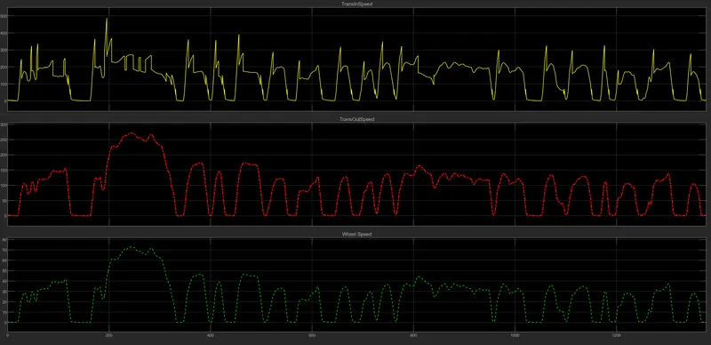
Here,We Are using Transmission Input and Transmission Output and Wheel Speed used for plotting The graph. transmission Output and Wheel Speed gives the same output

and we are using some saturation points to limit the graph movement.

Fuel Consumption vs Fuel Flow Rate vs Engine torque Vs Engine Power/Speed

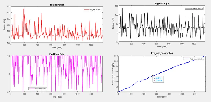
In UDDS cycle the Fuel Consumnption is high it goes upto 400 g/s and we using subplot command to plot the qudrant graphs in single figure.

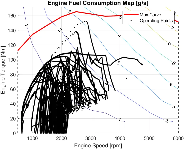
Engine Fuel Consumption (UDDS Drive cycle):

\

In this graph the dark black lines are the fuel consumption points and maximum torque starts from 1000 rpm and it gets peak in 3000- 4000 rpm and colour line sshown in the graph mentions the ranges of fuel consumption points.

Accelerator and brake pedal, gear command, vehicle desired and actual speed, vehicle distance

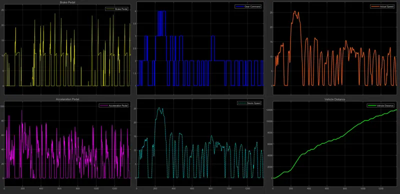
here,We are combining 6 graphs at one place using goto block and make visible at global and scope block is used to fetch the graph. The UDDS cycle runs upto 1380 sec.Here the graph getting peak at 200-400 sec.

HWFET Cycle:

%%%%%%%%%%%%%%%%%%%%%%%%%%%%%%%%%%%%%%%%%%%%%%%%%%%%%%%%%%%%%%%%%%%%%
%% Skill-Lync -> Hybrid Drives Development
% Project 1 - Conventional Vehicle Model
% By - Ullekh Gambhira 

% Description:

%% Initialization File
% Initialization file for loading the variables for the Conventional vehicle simulation model

%% Vehicle Parameters
M = 1500;       % Vehicle weight [kg]
Cr = 0.015;     % Rolling resistance coefficient
Rw = 0.35;      % Rolling radius [m]
Cd = 0.33;      % Drag coefficient
Af = 2;         % Frontal area [m2]
rhoa = 1.225;   % Air density [kg/m3]
Vwind = 0;      % Wind velocity [kmph]
g = 9.81;       % Gravitational acceleration [m/s2]
theta = 0;      % Slope [deg]
myu_road_tire = 1; % Coefficient of friction between tire - road interface
set_param('Project1_VehicleModel_FINAL','DataTypeOverride','Off');

%% Powertrain Parameters 
FDR = 3.73;                         % Final Drive Ratio / Diff Ratio
DiffEff = 0.99;                     % Differential efficiency (assumed independent of operating conditions)

NumGear = 4;                        % Number of gears in transmission
TransGear = [1:NumGear];            % Transmission Gears
TransRatio = [3.06, 1.62, 1, 0.7];  % Corresponding Transmission ratios
TransEff = 0.90;                    % Transmission efficiency (assumed independent of operating conditions)

TC_SR = [0, .5, .6, .7, .8, .87, .92, .94, .96, .97, 1];   % Torque Converter Speed Ratio (Matlab default) -> TurbSpd/PumpSpd  
TC_TR = [2.232, 1.5462, 1.4058, 1.2746, 1.1528, 1.0732, 1.0192, 1, 1, 1, 1];   % Torque Converter Torque Ratio (Matlab default) -> TurbTrq/PumpTrq
TC_Cf = 1e-4 * [.72558, .66322, .63463, .59042, .51331, .4144, .29287, .22444, .12186, .04386, 0]; % Torque Converter Capacity Factor (Matlab default) -> PumpTrq/PumpSpd^2 [Nm/rpm^2]

load Vehicle_Data/Engine_data_1_9L_Saturn_95kW
load Vehicle_Data/Trans_Shift_map

%% Driver Parameters
Kp = 10;                    % P gain for driver PI model
Ki = 1;                     % I gain for driver PI model
Drive_Cycle_Select = 2;     % Drive cycle selection

% Drive cycle values in m/s

if Drive_Cycle_Select == 1
    load DriveCycles/UDDS;
    
elseif Drive_Cycle_Select == 2
    load DriveCycles/HWFET;
    
elseif Drive_Cycle_Select == 3
    load DriveCycles/FTP;
    
elseif Drive_Cycle_Select == 4
    load DriveCycles/US06;
    
elseif Drive_Cycle_Select == 5
    load DriveCycles/NEDC;
    
elseif Drive_Cycle_Select == 6
    load DriveCycles/WLTP;
 
end

time_end = cyc_time(end);
vel_end = cyc_vel(end);

time trace for engine, transmission input, transmission output and wheel speed on one plot

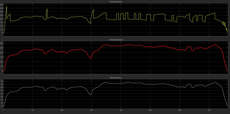
Here,Transmission input Speed and Transmission output Speed with Wheel Speed as same output with time range 765 sec.

engine torque, engine power, fuel rate and fuel consumption using subplots

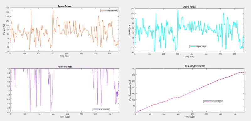
In HWFWT cycle the Fuel Consumnption is moderate and constant at some places and Engine power and Engine Torque Both graphs are follwing same pattern.we using subplot command to plot the qudrant graphs in single figure

Engine operating points on the engine fuel map and Fuel Consumption graph:

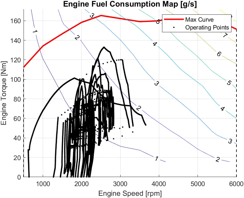
In this graph the dark black lines are the fuel consumption points and maximum torque starts from 1000 rpm and it gets peak in 3000- 4000 rpm and colour line shown in the graph mentions the ranges of fuel consumption points and Efficiency of the Engine.

Accelerator and brake pedal, gear command, vehicle desired and actual speed, vehicle distance

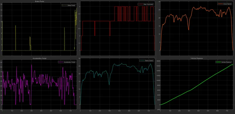
here,We are combining 6 graphs at one place using goto block and make visible at global and scope block is used to fetch the graph. The HWFET cycle runs upto 765 sec.Here the graph getting peak at 600-770 sec.

Simulink File:

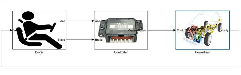
Here In the simulink block Forward Model with contineous Flow with comparing the output with the input to meet the desired Speed Range. There are Main three blocks are used here is Driver,Controller and Powertrain. In the powertrain block there are Svereal Subblocks are used That is Engine,Transmission,Differential,Wheel and Vehicle Dynamics and Output we are getting is Velocity/Speed of the vehicle.This will provide as Input for the Driver block.

Driver Block:

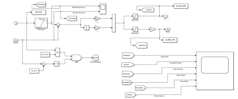
In the Driver block there is the starting part of the Vehicle Design many inputs and values have been created from here.Like Engine testing time,Acceleration Pedal,Brake Pedal,Vehicle Desired Speed and Actual Speed. There is Using And Logic gate and Saturation Blocks are used. The Saturation Block is mainly Used for Controlling the Graph by placing the Upper limit and Lower Limit.

Controller Block:

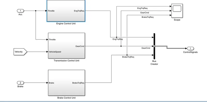
In the Controller Block There is 3 Important Subsystems are present.Engine Control unit, Transmission control,Brake Control units are avilable the Inputs are Acceleration pedal,Velocity,Brake Pedal and Output is combined into Control Signals.

Engine Control Unit:

Transmission Control unit:

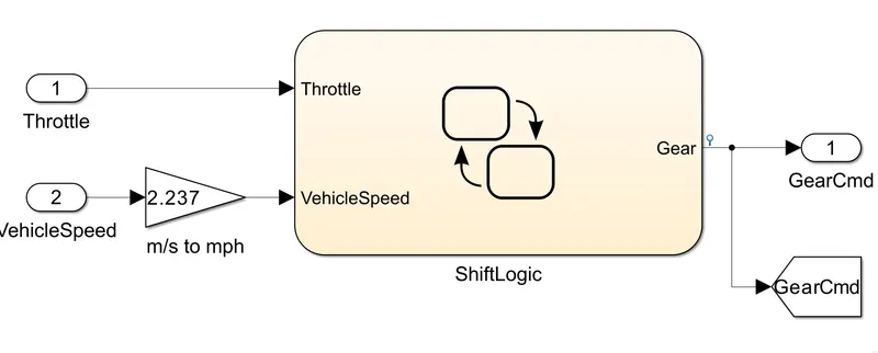
In the Transmission Control UNit there is gearshifting is there,so we change the gear shifting based on throttle and the output is Gear command and inputs are Vehicle Speed and Throttle.

Brake Control unit:

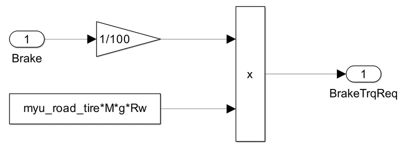
Brake control unit is the Simple Unit it multiplies Road load into Brake Pedal input and converts into Braketorque.

Power Train Block:

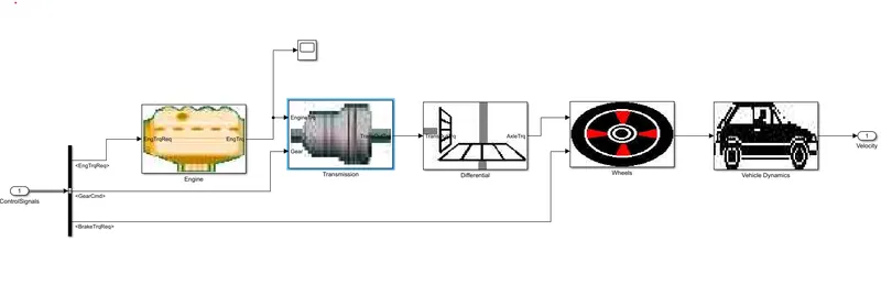
IN Powertrain Block There is Series of Subsystem Are Available Like Engine,Transmission,Differential,Wheel,Vehicle Dynamics.The Output of Every block is connected to the input for the next block.This will transmit the Energy from Engine to the Wheels and drive the Vehicle by Driver INput.

Engine Block:

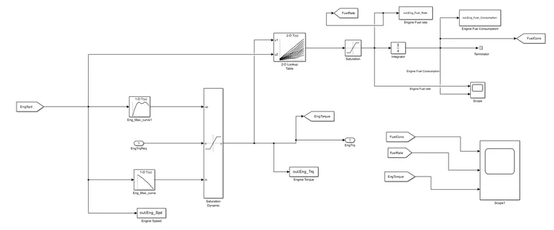
Engine Block there are many 1D and 2D Lookup tables are avilable lookup table are used to compare the values with refernce values and convert the raw data into Easy undertanding manner. The Engine Speed is the input of this block and output is Engine Torque and We are measuring Fuel flow rate and Fuel consumption. There is neede to plot the Fuel Consumption graph.

Transmission Block:

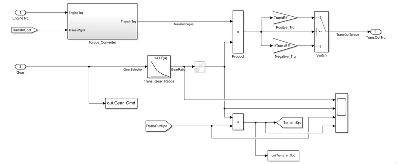
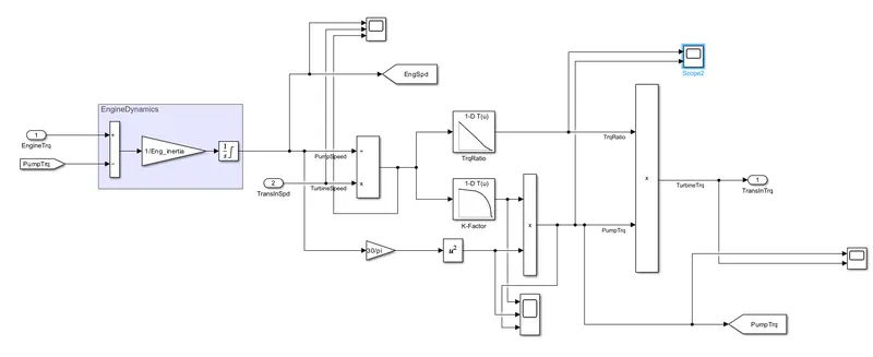
here,Transmission Block there is Torque Convereter is used inside the torque converter there are many blocks are available Like Pumptorque ,Turbine torque,Engine Speed are avilable the Transmission Torque is the output of the Torque Converter.

torque convereter:

Differential Block:

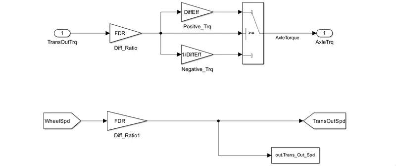
Here,Transmission Torque and Wheel Speed as a input for this block wheel speed we are getting from wheels subsystem and using global visibility goto block.we are getting Transoutput Speed from Wheel Speed and Axle trq from Transouttrq.

Wheel Block:

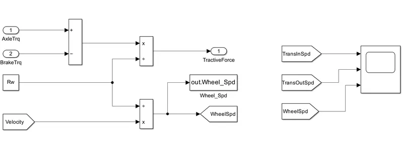
Here,Axle and Brake torque as the Inputs of this block and Roadload velocity is being mutiplied to get the Wheel Speed and Tractive Force.

Vehicle Dynamics Block:

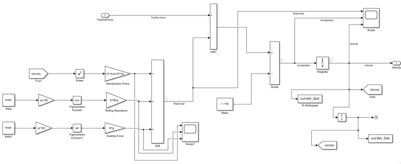
here Vehicle dynamics Block we are using rolling resistance,Aerodynamic Resistance and Grading Force added with specific blocks and combine into tractive Force input and final output we are getting Velocity which will Comparing with the Driver unit.