Project 2
Project - 2
Aim : Develop a model for forwarding Energy based fuel consumption model of a P1 type Hybrid Vehicle.
Goal : To understand the functionality of a P1 hybrid and be able to model it.
Objective :
a. Tabulate the fuel economy numbers (kmpl) for UDDS and HWFET cycle. Compare these numbers with the baseline numbers for conventional vehicle model from Project 1.
b. Plot the time trace for engine, transmission input, transmission output and wheel speed on one plot.
c. Plot engine torque, engine power, fuel rate and fuel consumption using subplots.
d. Plot accelerator and brake pedal, gear command, vehicle desired and actual speed, vehicle distance using subplots.
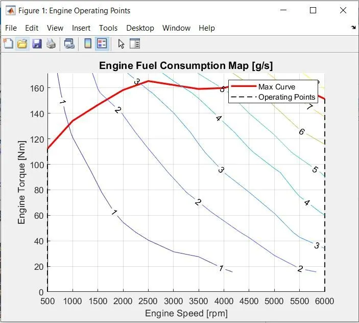
e. Plot the engine operating points on the engine fuel map.
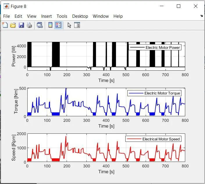
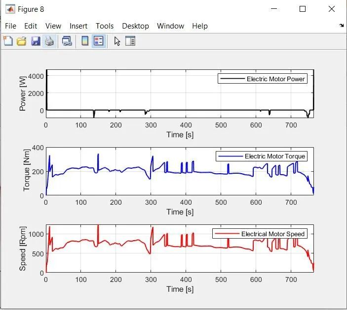
f. Plot motor speed, torque, motor input power using subplots.
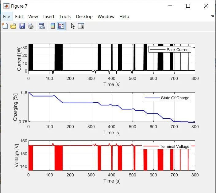
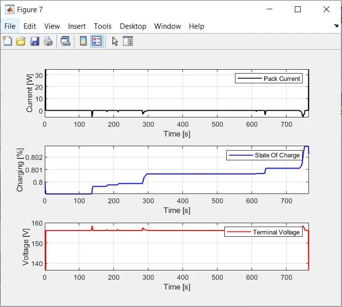
g. Plot pack voltage, current and SoC using subplots.
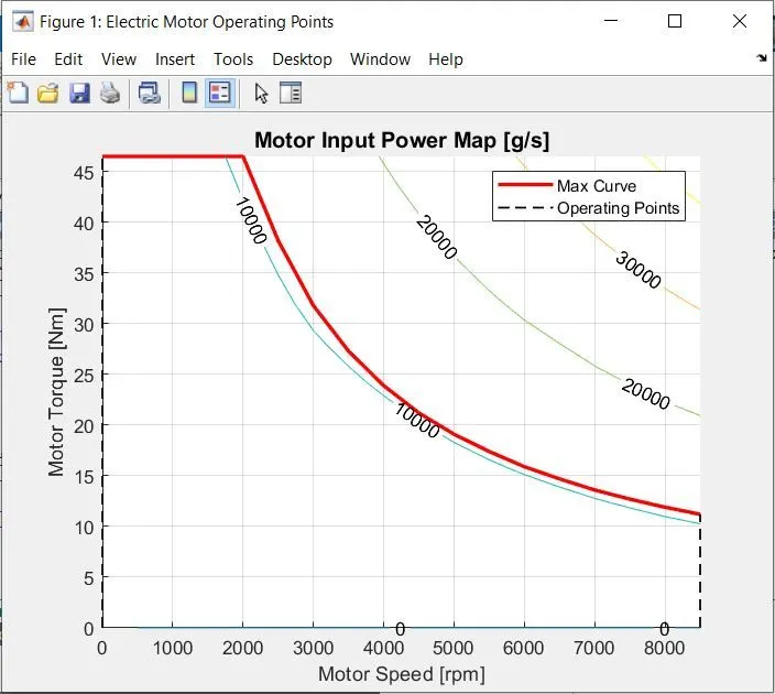
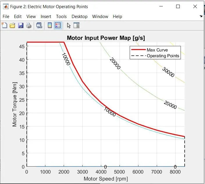
h. Plot the motor operating points on the motor input power map, with the motor max motoring and generating torque curves.
i. Write down appropriate brief comments on each of these plots, describing the vehicle behavior throughout the drive cycle.
j. Generate the plots for both drive cycles
Hybrid Vehicle Architecture :
There are three main types of hybrid vehicle; full hybrids, mild hybrids and plug-in hybrids.
By architecture, topology or configuration we understand the positioning of the main components of the hybrid electric system on the vehicle. Since the only mechanical link between the electrical system and the rest of the vehicle is done through the electric machine, the MHEV architecture is basically defined by the position of the electric machine and the type of connection with the powertrain / drivetrain (belt, integrated or gear mesh).
The 48V electrical system has become the industry standard for mild hybrid MHEV applications for several reasons:
- it’s relatively simple to integrate on a vehicle
- it’s modular, safe and compact
- the mass of the components is relatively small so the impact on the total weight of the vehicle is limited
- the system cost to performance (fuel efficiency, torque boost) ratio is very competitive
With the except of the crankshaft-mounted integrated starter generator (Honda IMA and Mercedes Benz BlueHybrid), all the mild hybrid vehicle architectures presented in this article are based on 48V systems.
The powertrain configuration of the MHEV system has significant impact on the performance and characteristics of the vehicle, in terms of:
- integration cost
- fuel efficiency
- dynamic performance (powertrain torque enhancement)
Automotive OEMs and automotive Tier 1 system suppliers are currently analyzing and evaluating several major powertrain architectures for MHEVs. The electric machine can be positioned, relative to the other powertrain components, in five major points:

Image: MHEV powertrain architectures
The brief description of the electric machine connection points is done in the table below.
| P0 | The electric machine is connected with the internal combustion engine through a belt, on the front end accessory drive (FEAD) |
| P1 | The electric machine is connected directly with the crankshaft of the internal combustion engine |
| P2 | The electric machine is side-attached (through a belt) or integrated between the internal combustion engine and the transmission; the electric machine is decoupled from the ICE and it has the same speed of the ICE (or multiple of it) |
| P3 | The electric machine is connected through a gear mesh with the transmission; the electric machine is decoupled from the ICE and it’s speed is a multiple of the wheel speed |
| P4 | The electric machine is connected through a gear mesh on the rear axle of the vehicle; the electric machine is decoupled form the ICE and it’s located in the rear axle drive or in the wheels hub |
Notice that P0 and P1 architectures do not allow the mechanical disconnection of the electric machine from the engine. On the other side P2, P3 or P4 configurations disconnects the electric machine from the engine through a clutch.
Crankshaft mounted electric machine (P1)
The P1 architecture, with the electric machine connected directly to the crankshaft, is the solution adopted by Honda on their first generation Integrated Motor Assist (IMA) technology. The electric motor functions as a generator, during vehicle deceleration, as an engine starter, and as a motor (to assist the engine) during vehicle accelerations.

Image: MHEV P1 architecture – Integrated Starter Generator (ISG)
One of the biggest advantage of this solution is that the electric motor can provide higher torque than the BiSG, since there is no belt limitation (due to slip). However, since there is no speed / torque ratio between the electric machine and crankshaft, the torque requirements on the electric motor can be quite demanding.
Two examples of P1 MHEV architectures are:
- Honda Insight Hybrid 2009 (with Integrated Motor Assist technology)
- Mercedes Benz S400 Bluehybrid 2010

Image: Integrated Motor Assist (IMA) for mild hybrid
Credit: Honda
For example, the main characteristics of the crankshaft-mounted electric machine for mild hybrid Honda Insight 2009 are summarized in the table below.
| Electric machine performance | Maximum torque (at crankshaft): up to 34 Nm Maximum power: 10 kW Efficiency: up to 94% |
| Hybrid modes (functions) | Idle Stop & Start Moving Stop & Start Engine load shift Torque assist (fill) Torque boost Sailing / Coasting Energy recuperation Brake regeneration |
| Advantages | Higher efficiency The 12V starter can be removed |
| Disadvantages | Output torque limited by the size of the electric machine Energy recuperation affected by engine friction losses High impact on existing vehicle architecture Higher overall cost of the electrical components Air cooling not possible for the electric machine |
| Overall characteristics | Torque Boosting Capability: High (if electric machine is capable) Electrical Energy Recuperation: Medium (due to engine losses) Driveability Improvements: Medium (depending on the torque capability of the electric machine) Electrical Creep / Drive: Possible (depending on the torque capability of the e-machine) Packaging: Difficult components integration (powertrain specially designed for this architecture) System Efficiency: High (no gear mesh or belt losses) |

Image: Mercedes Benz S400 BlueHybrid (MHEV)
Credit: Daimler
The primary advantage of a P1 mild hybrid architecture, compared with P0, is the removal of the belt drive. This means that the efficiency increases a bit (no more belt losses) and the electric machine torque can be higher in terms of amplitude and response (no more belt slip).
The functions (modes) performed by this mild hybrid topology are similar with those of a BiSG (P0), but, overall, P1 configurations have two big disadvantages: higher cost and higher impact on the the existing vehicle architecture. Therefore, vehicle manufacturers and system suppliers are not investing in the further development of crankshaft-mounted integrated starter generator solution for MHEV applications.
Forward modeling of Vehicle :
Forward-facing models represent dynamic models with the correct causality. A forward-facing vehicle model features a driver model, which provides torque demand in the form of desired ICE torque and brake torque (positive and negative torque), to meet the speed trace from a drivecycle.
- This approach is based on the vehicle dynamics equation.
- A Driver Controller is required to control the vehicle to follow desired speed and to calculate.
- The Controller is implemented to model that the driver will either push the accelerator or the brake pedal to match the desired speed which enables to study the braking of the vehicle
- It also acts as a feedback loop for the vehicle which was used to determine the energy requirements to drive the vehicle.
Conventional Vehicle Model:
But we are using Hybrid Architecture in this model, so we want to build the model like the below image,
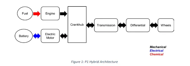
In this project, we have the instructions to follow in steps. Because of this, the Simulation will process in 3 stages.
- Project Initialization (Pre Processing)
- Simulation
- Post processing
Pre Processing :
In this Stage data which load as a program, it will take as an input program of the vehicles which is used for Post-processing of the Simulation by using the Simulink Model which is already built
Drive Cycle selection is also done from here by choosing the variable in it eg:1 is for UDDS, 2 is for HWFET, and 3 is for FTP.
Then we want to write the initial parameters data of the Vehicle Dynamics is Consists of a typical 4-gear vehicle.
Drive Cycle which was used in this program is US-based Vehicles Dynamics
By the Changing the variable input for selecting different Drive_cycle
1 UDDS
2 HWFET
3 FTP
4 US06
5 NEDC
6 WLTP
Simulink Modeling :
The Model of Simulink is for the convection model of the vehicle in which it has been divided into 3 main sub-blocks are:
- Driver
- Controller
- Powertrain
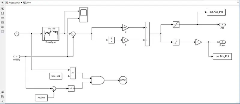
The Actual Vehicle speed is given as feedback to the driver block, and the driver block gives into the controller block in which the acceleration or brake output is connected.
While the controller provides a control signal for engine torque, gear shifting, and brake torque to the powertrain block.
The PI controller controls the error between the required drive cycle and the actual vehicle speed is been provided by the acceleration and brake pedal output of the controller unit.
Controller :
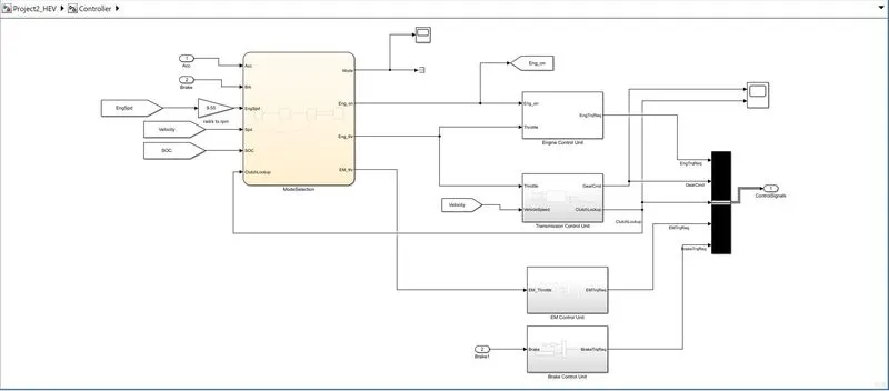
The control request from the driver block is fed into the controller block and based on this different control action is performed. The controller block consists of a master controller, Engine control unit, Brake control unit, Transmission Control unit and motor control unit. From the master control unit different signal is send to the other controller to perform action according to the modes. The figure shows the controller unit for P1 hybrid model.
Master Control Unit :
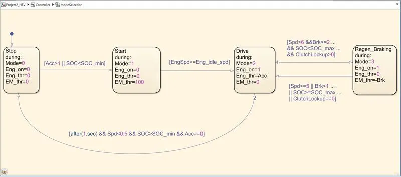
Master control unit is the main control unit for hybrid vehicle.This control unit decides which operation/modes the vehicle should be in. For P1 hybrid two features have been intrgrated i.e. Start and stop and regenerative braking.The figure 6 shows the controller logic and based on the input like accleration, braking, Soc level, vehicle speed different modes is selected.
Engine control Unit :
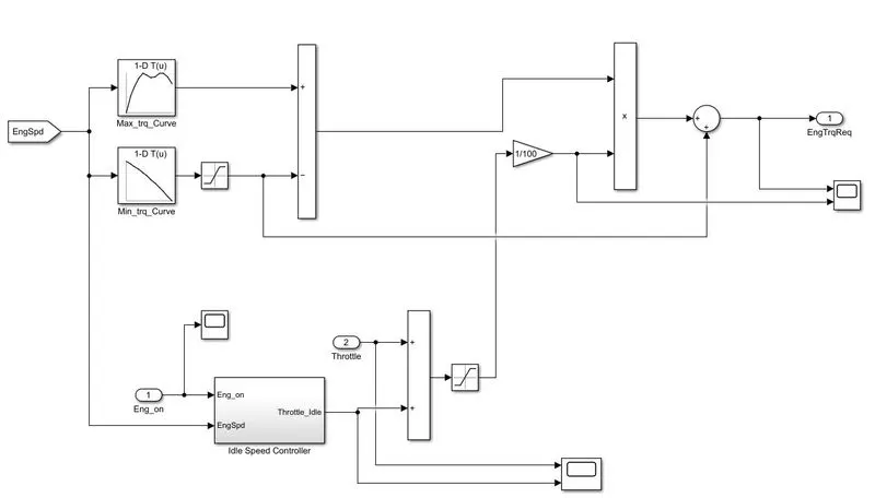
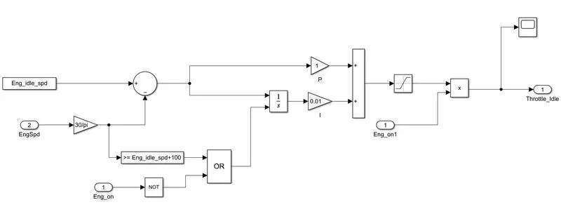
Based on the engine throttle coming from the master controller, a torque request is supplied to the powertrain blockset. To integrated idle start stop feature, a variable called as engine on is used which value is 0 for engine off and 1 for engine on. The value of engine on is determined by the master controller based on the modes which the vehicle is in. This helps to save fuel when the vehicle is in idling. Figure shows the engine control unit used for this project.
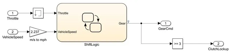
This Control unit has 2 inputs whereas Throttle, Vehicle Speed, and Gear Command as Output.
Has Increasing the Input Throttle speed, Changing of gear commands take place accordingly 1,2,3,4 and vice versa for speed dropping condition.
In transmission control unit, based on the throtle request from the master controller and vehicle speed a gear command and clutch lock up command is generated. This command is generated based on the control logic/transmission shift logic define by using the state flow.
Gear Selection :
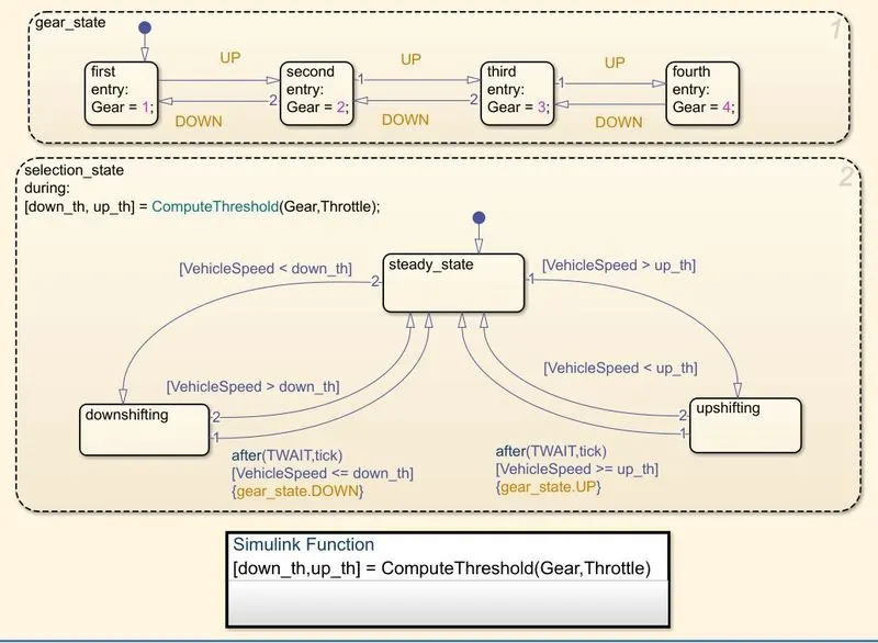
The Gear command is been created by using the Stateflow block for this simulation.
It is been controlled accordingly by Vehicle Speed and Throttle inputs.
The gear command is been passed to the transmission block to select the desired gear ratio.
Electric Motor Control Unit :
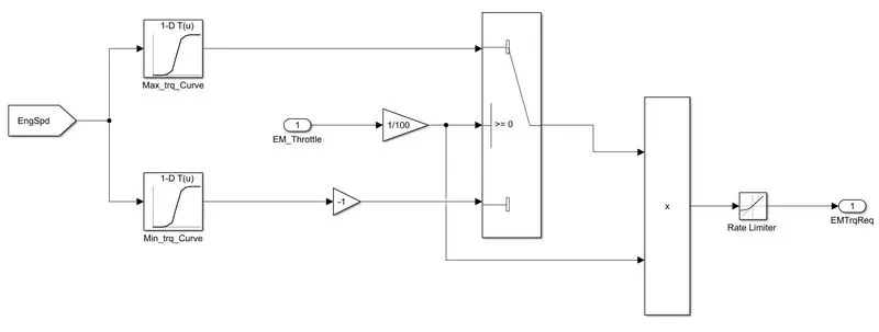
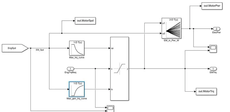
In this unit, motor throttle request is fed in as an input, and based on the speed of motor and throttle, either motoring torque or generating torque is selected from the look-up table. This torque is multiplied to get the electric motor torque request. Since the engine is integrated wi the electrical machine, the speed of an engine is taken as an input speed for a motor. The figure shows the Motor control unit.
Brake Control Unit :
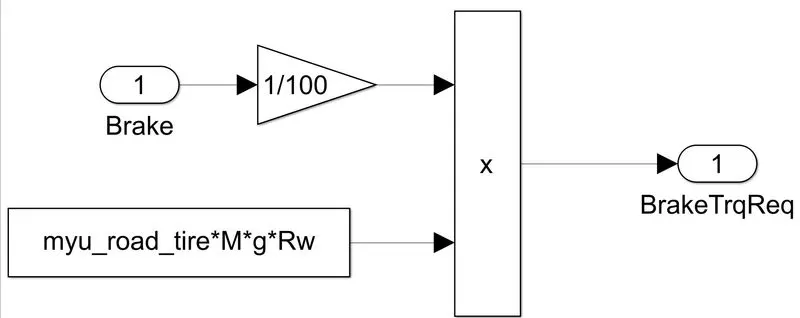
In this control unit, the braking request from the driver is fetch as an input and based on the braking action of the driver brake torque request is send to the driver.Figure 11 shows the barke control unit used in this project.
All this control signal from the controller is fetch to the bus creator , which merges the signal and send it to the powertrain block.
Powertrain :
A powertrain is a system inside a vehicle, boat or another type of machinery. The system is designed to propel the vehicle forward. In a car, a powertrain consists of the engine or motor and its internal components, such as the energy storage system, transmission and driveshaft.
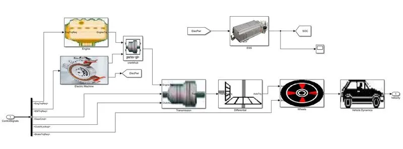
In powertrain we consists for Engine block, transmission block, differential block, Motor, battery, Wheels and vehicle body.The control signal form the controller block is send to the powertrain block and based on which the velocity of the vehicle is determined.
Engine Block :
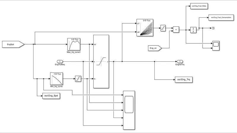
In this block based on the engine speed and torque request from the controller, fuel consumption is taken out by using a lookup table,The torque from the engine is also calculated based on the torque request and engine speed and based on the torque engine speed is also calculated at the transmission block.
Electric Machine :
In motor subsystem also, based on the the motor torque request from the controller and engine speed the torque and input power to the motor is calculated. The engine speed is considered because it is considered that engine and motor are running at the same speed in P1 hybrid Vehicle.
Battery :
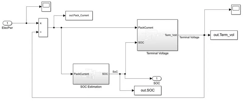
In battery subsystem,based on the input power demand from the motor, the current from the battery is considered. And based on the current drawn , SOC level of the battery is calculated by considered the technique called as columb counting. The Voltage of the battery being the function of the SOC level of the battery, so the open circuit voltage is calculated by SOC level of battery.
Crank hub :
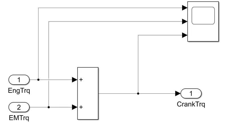
This block is used to compute the both output from the Engine and E-Motor Power into a Single Output to supply its Transmission System.
Transmission :
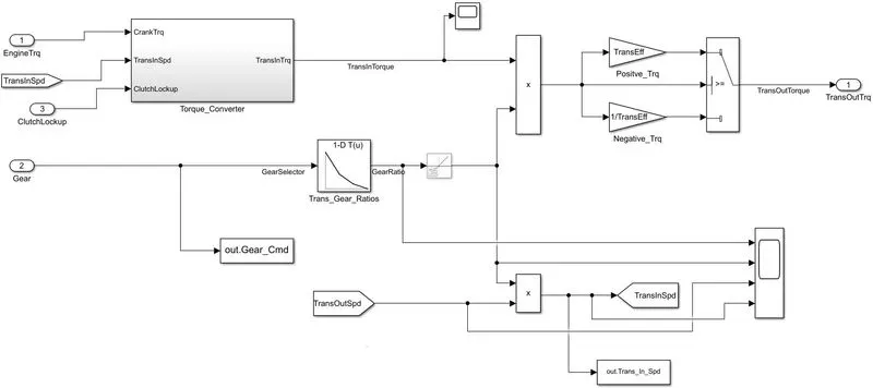
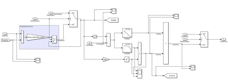
In the transmission subsystem based on the input crank torque and Transmission speed, the torque from the torque converter is calculated. Based on the gear command from the controller, the gear ratio is selected by considering the gear and gear ratio data from the lookup table, product of gear ratio and torque from the torque converter gives us the total output torque from the transmission. Based on the nature of torque its efficiency is assigned and output torque is calculated.
Torque Converter:
A torque converter is a type of fluid coupling that transfers rotating power from a prime mover, like an internal combustion engine, to a rotating driven load. In a vehicle with an automatic transmission, the torque converter connects the power source to the load. It is usually located between the engine's flexplate and the transmission. The equivalent location in a manual transmission would be the mechanical clutch.
Differential:
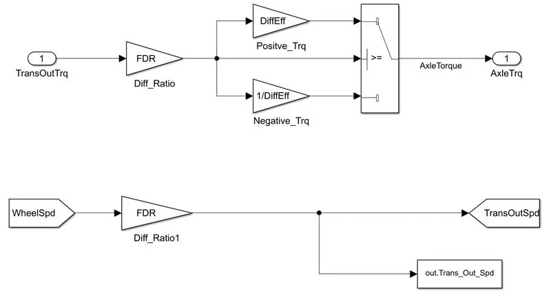
In the differential subsystem, the transmission output torque is multiplied by the final drive ratio of the system, and based on the nature of the torque, negative or positive axle torque is calculated.
Wheels :
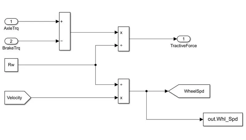
In wheel subsystem, the brake torque request from the brake contoller is fetch in. Based on the brake torque request and axle torque, traction force is calculated by considering the wheel speed. And the traction force is send to the vehicle body subsystem.
Vehicle Dynamics:
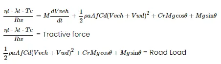
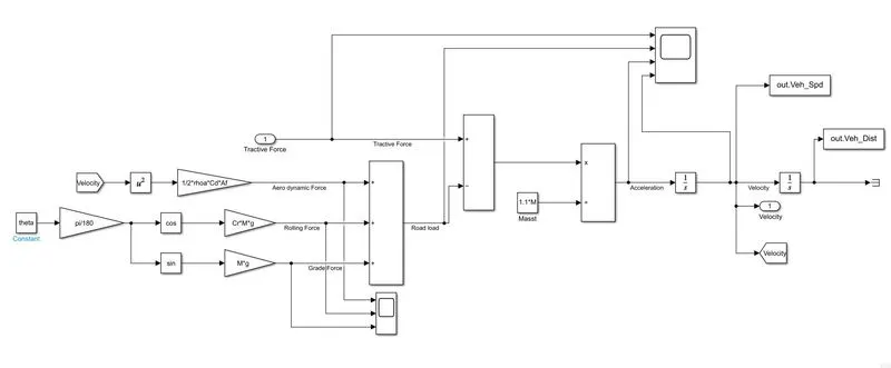
This block consists of the longitudinal dynamics of the vehicle which consists of Aerodynamics force, Rolling Resistance Force, Grade Force etc..,
Formulas used:
Post-Processing :
Result:
The model had been run for the different cycles and different parameters were analyzed and compared with the conventional vehicle model.
Comparision for Different Drive Cycle:
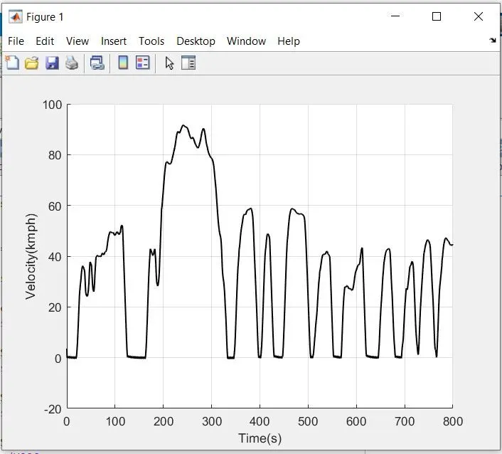
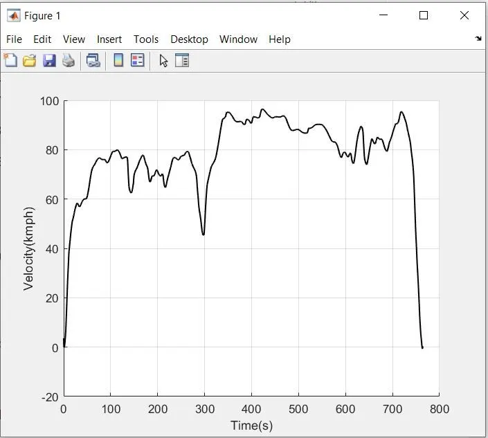
Two drive cycles UDDS and HWFET were considered and different system level parameters were analyzed.
UDDS :
HWFET:
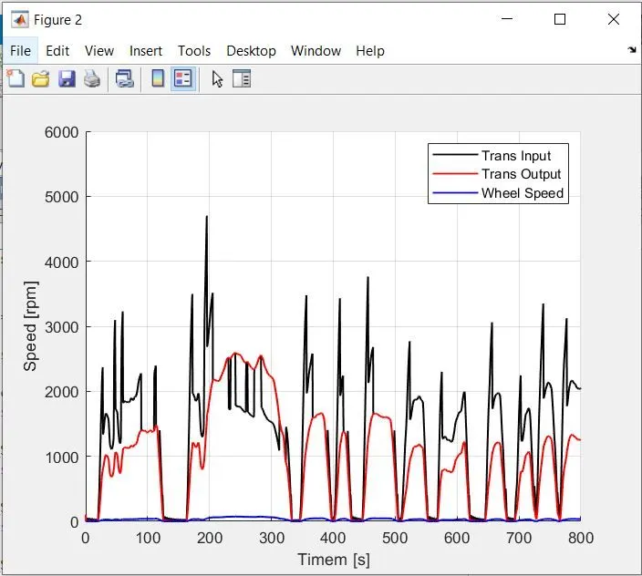
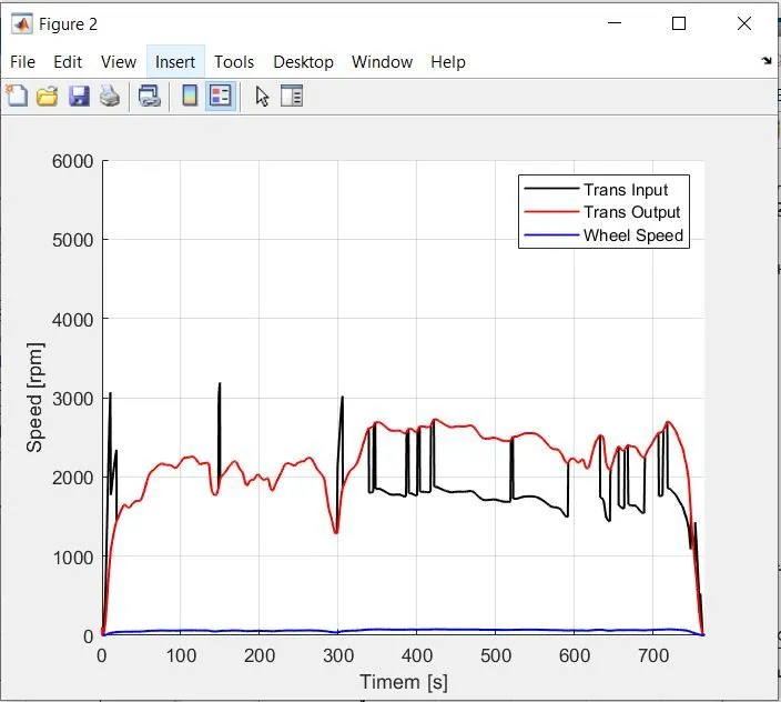
b. Plot the time trace for engine, transmission input, transmission output and wheel speed on one plot.
Comparision for Speed for engine, wheel, and Transmission for both Drive cycles:
The below figure shows the speed of the engine wheel and transmission system for the UDDS cycle while Figure shows the same for the HWFET cycle. In the UDDS cycle, we can observe the average speed of the wheel transmission and the engine is higher in the case of the HWFET cycle as the vehicle has to propel with higher velocity as compared with the UDDS cycle. It was also observed that in the UDDS cycle, there is a more frequent rise and fall in the speed of the wheel, engine, and transmission than in the HWFET cycle. This is due to the frequent stop-start condition in urban driving conditions.
UDDS :
HWFET :
c. Plot engine torque, engine power, fuel rate and fuel consumption using subplots.
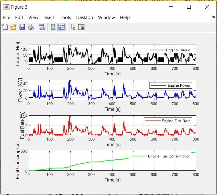
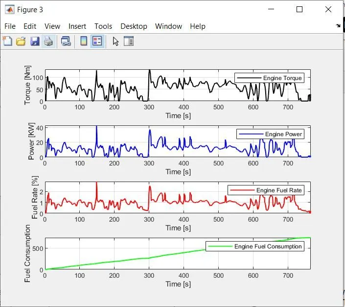
Engine Analysis for HWFET cycle and UDDS cycle:
In the UDDS cycle, we can observe that there is a frequent rise and fall in engine power and torque while for the HWFET cycle, the fall and rise are comparatively smaller than in the UDDS cycle as shown in figures 23a and 23b. This enables the HWFET cycle to work in a more efficient region as compared with the UDDS cycle which lowers the fuel consumption rate. The highest fuel consumption rate for the UDDS cycle is around 4 gm/sec, while for the HWFET cycle it is around 3.2 gm/sec. The HWFET cycle works more in a higher efficient region when compared with the UDDS cycle. In the HWFET cycle, we can observe the minimum amount of negative torque from the engine when compared with the UDDS cycle, in highway vehicles need not have to deal with frequent start-stop conditions. At the end of the drive cycle, the overall consumption was around 700 gm for the HWFET cycle and around 600 gm for the UDDS cycle.
UDDS :
HWFET :
d. Plot accelerator and brake pedal, gear command, vehicle desired and actual speed, vehicle distance using subplots.
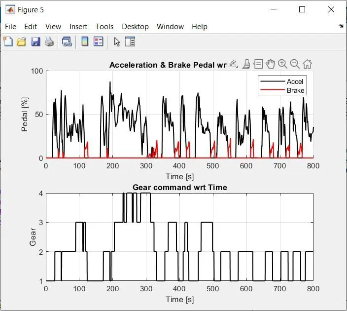
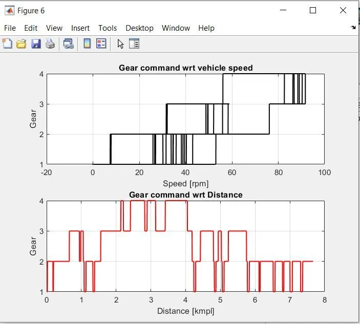
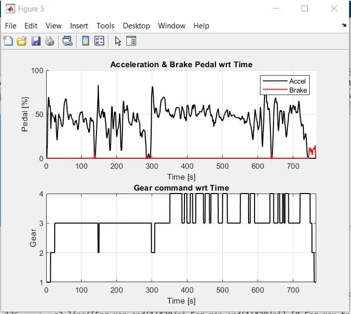
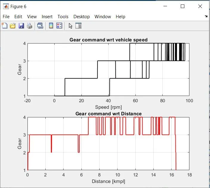
Accelerator, Brake pedal position, and Gear Selected for different drive cycle
The below figure shows the brake pedal and accelerator pedal position for the UDDS cycle. We can observe that when the vehicle is following the UDDS cycle the use of the brake pedal is quite often and the intensity for the pedal is pressed is also high as compared with the HWFET cycle in figure 24b. The vehicle is often in a higher gear for the HWFET cycle as compared with the UDDS cycle. The vehicle has covered a distance of around 12 km for the UDDS cycle and around 17km for the HWFET cycle.
UDDS :
HWFET :
e. Plot the engine operating points on the engine fuel map.
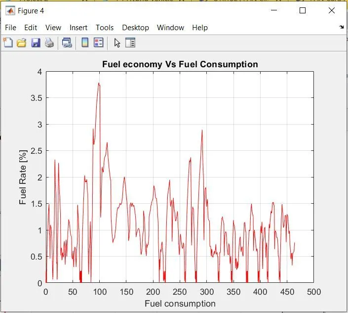
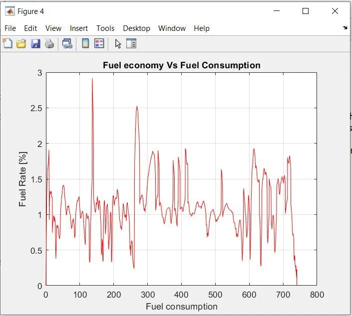
Fuel Economy Vs Fuel Comsumption:
UDDS :
HWFET :
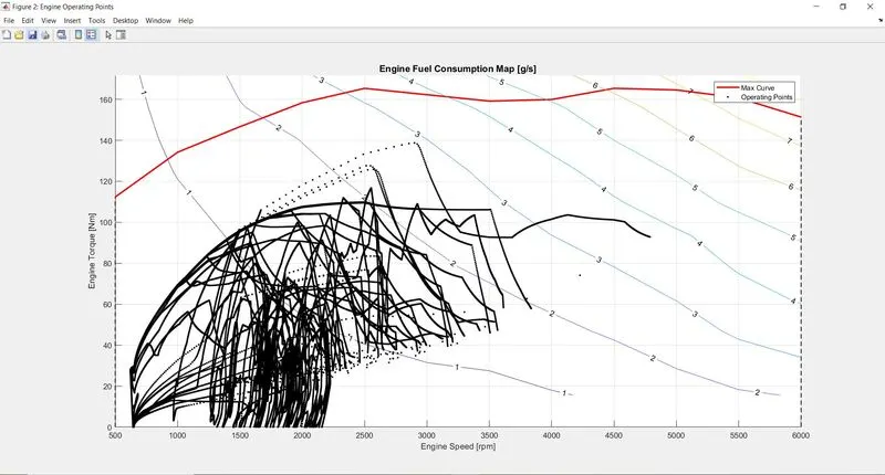
Comparison of Fuel Consumption Map of Convectional vehicle vs P1 Hybrid Vehicle:
UDDS:
Figure a)Engine performance map with its operating point for conventional vehicles in the UDDS cycle.b) Engine performance map with its operating point for Hybrid Vehicle For UDDS
for the hybrid vehicle in the UDDS.
Conventioinal Vehicle -UDDS :
UDDS :
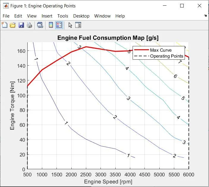
HWFET Vs Conventional Vehicle :
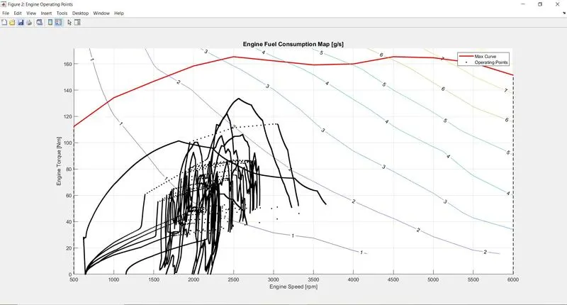
The below figure shows the Engine performance map with its operating point for conventional vehicles in the HWFET cycle.b)Engine performance map with its operating point for the hybrid vehicle in the HWFET cycle.
Conventional Vehicle - HWFET :
HWFET :
f. Plot motor speed, torque, motor input power using subplots.
Comparison Of Electric Motor of Speed, Torque , Power vs Time:
UDDS :
HWFET :
g. Plot pack voltage, current and SoC using subplots.
Pack Current, State Of Charge, Terminal Voltage vs Time:
UDDS :
HWFET :
h. Plot the motor operating points on the motor input power map, with the motor max motoring and generating torque curves.
Plot the motor operating points on the motor input power map, with the motor max motoring and generating torque curves.
UDDS :
HWFET :
Conclusion:
The system-level analysis were done for the given Honda Insight P1 Hybrid model vs Convectional Vehicle.
And the required plot results are shown above.