Project
All-Terrain Vehicle -
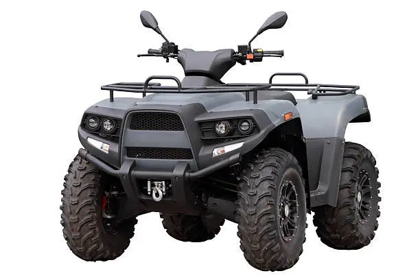
Fig:1 All-Terrain Vehicle (ATV)
An all-terrain vehicle (ATV), also known as a light utility vehicle (LUV), a quad bike, or simply a quad, as defined by the American National Standards Institute (ANSI); is a vehicle that travels on low-pressure tires, with a seat that is straddled by the operator, along with handlebars for steering control. As the name implies, it is designed to handle a wider variety of terrain than most other vehicles. Although it is a street-legal vehicle in some countries, it is not street-legal within most states, territories, and provinces of Australia, the United States, or Canada.
By the current ANSI definition, ATVs are intended for use by a single operator, although some companies have developed ATVs intended for use by the operator and one passenger. These ATVs are referred to as tandem ATVs.
The rider sits on and operates these vehicles like a motorcycle, but the extra wheels give more stability at slower speeds. Although most are equipped with three or four wheels, six-wheel models exist and existed historically for specialized applications. Multiple-user analogs with side-by-side seating are called utility terrain vehicles (UTVs) or side-by-sides to distinguish the classes of vehicles. Both classes tend to have similar powertrain parts. Engine sizes of ATVs currently for sale in the United States (as of 2008 products) range from 49 to 1,000 cc (3.0 to 61 cu in).
Continuously Variable Transmission (CVT) -
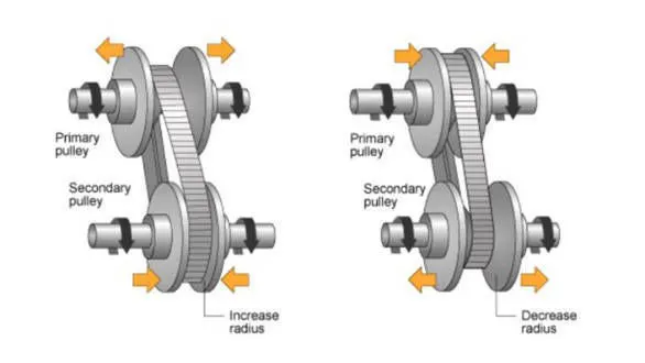
Fig:2 Continuously Variable Transmission (CVT)
A continuously variable transmission (CVT) is an automatic transmission that can change seamlessly through a continuous range of gear ratios. This contrasts with other transmissions that provide a limited number of gear ratios in fixed steps. The flexibility of a CVT with suitable control may allow the engine to operate at a constant RPM while the vehicle moves at varying speeds.
CVTs are used in automobiles, tractors, motor scooters, snowmobiles, bicycles, and earthmoving equipment.
The most common type of CVT uses two pulleys connected by a belt or chain; however, several other designs have also been used at times.
Blocks:-
- Circular Gauge -

The Circular Gauge block displays the value of the connected signal on a circular gauge that you can design to look like a gauge in a real system.
The Circular Gauge block displays the instantaneous value of the connected signal throughout the simulation. You can modify the range and tick values on the Circular Gauge block to fit your data. Use the Circular Gauge block with other dashboard blocks to build an interactive dashboard of controls and indicators for your model.
- Knob -

The Knob block tunes the value of the connected block parameter during simulation. For example, you can connect the Knob block to a Gain block in your model and adjust its value during simulation. You can modify the range of the Knob block's scale to fit your data. Use the Knob block with other Dashboard blocks to create an interactive dashboard to control your model.
- Constant -

Output the constant specified by the 'Constant value' parameter. If 'Constant value' is a vector and 'Interpret vector parameters as 1-D' is on, treat the constant value as a 1-D array. Otherwise, output a matrix with the same dimensions as the constant value.
- Goto -

The Goto block passes its input to its corresponding From blocks. The input can be a real- or complex-valued signal or vector of any data type. From and Goto blocks allow you to pass a signal from one block to another without actually connecting them.
A Goto block can pass its input signal to more than one From block, although a From block can receive a signal from only one Goto block. The input to that Goto block is passed to the From blocks associated with it as though the blocks were physically connected.
- From -

The From block accepts a signal from a corresponding Goto block, then passes it as output. The data type of the output is the same as that of the input from the Goto block. From and Goto blocks allow you to pass a signal from one block to another without actually connecting them.
- Simulink-PS Converter -

Converts the Simulink input signal to a Physical Signal.
The unit expression in the 'Input signal unit' parameter is associated with the Simulink input signal and determines the unit assigned to the Physical Signal.
- PS-Simulink Converter -

The PS-Simulink Converter block converts a physical signal into a Simulink output signal. Use this block to connect outputs of a Simscape physical network to Simulink scopes or other Simulink blocks.
- Solver Configuration -

Each physical network represented by a connected Simscape block diagram requires solver settings information for simulation. The Solver Configuration block specifies the solver parameters that your model needs before you can begin the simulation.
Each topologically distinct Simscape block diagram requires exactly one Solver Configuration block to be connected to it.
- Mechanical Rotational Reference -

The Mechanical Rotational Reference block represents a reference point, or frame, for all mechanical rotational ports. All rotational ports that are rigidly clamped to the frame (ground) must be connected to a Mechanical Rotational Reference block.
- Generic Engine -
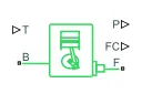
The Generic Engine block represents a general internal combustion engine. This block is a suitable generic engine for spark ignition and diesel. Speed-power and speed-torque parameterizations are provided. A throttle physical signal input specifies the normalized engine torque. Optional dynamic parameters include crankshaft inertia and response time lag. A physical signal port outputs the engine fuel consumption rate based on the fuel consumption model that you choose. Optional speed and redline controllers prevent the engine to stall and enable cruise control.
- Subsystem -
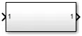
A Subsystem block contains a subset of blocks within a model or system. The Subsystem block can represent a virtual subsystem or a nonvirtual subsystem.
- Connection Port -

The Connection Port block transfers a physical connection or signal across subsystem boundaries. Physical connections include Simscape™ conserving connections and Simscape Multibody™ frame connections, among others. This block is similar in function to the Import and Outport blocks in the Simulink Ports & Subsystems library.
A subsystem needs a Connection Port block for each physical connection line that crosses its boundary. You can manually place a Connection Port block inside a subsystem, or Simulink can automatically insert a Connection Port block when you create a subsystem within an existing network.
- Ideal Rotational Motion Sensor -

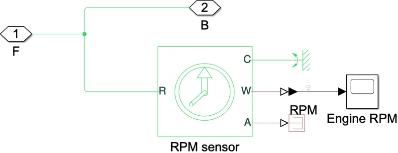
The Ideal Rotational Motion Sensor block represents an ideal mechanical rotational motion sensor, that is, a device that converts an across variable measured between two mechanical rotational nodes into a control signal proportional to angular velocity or angle. You can specify the initial angular position (offset) as a block parameter.
The sensor is ideal since it does not account for inertia, friction, delays, energy consumption, and so on.
Connections R and C are mechanical rotational conserving ports that connect the block to the nodes whose motion is being monitored. Connections W and A are physical signal output ports for velocity and angular displacement, respectively.
The block's positive direction is from port R to port C. This means that the velocity is measured as ω = ωR – ωC, where ωR, and ωC are the absolute angular velocities at ports R and C, respectively.
- PS Terminator -

Use the PS Terminator block to cap physical signal output ports that do not connect to other blocks.
Unlike conserving ports in physical modeling, or Simulink® output ports, unconnected physical signal output ports do not generate warnings. However, you can use a PS Terminator block for clarity, to indicate that the signal was not inadvertently left unconnected.
The block icon size allows you to connect the PS Terminator block to an open port without rerouting the adjacent lines:
- Scope -

Display signals generated during simulation.
- Signal Builder -
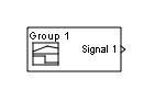
The Signal Builder block allows you to create interchangeable groups of piecewise linear signal sources and use them in a model. You can quickly switch the signal groups into and out of a model to facilitate testing. In the Signal Builder window, create signals and define the output waveforms. To open the window, double-click the block.
- Inertia -

The block represents an ideal mechanical rotational inertia.
The block has one or two mechanical rotational conserving ports. The difference is purely graphical, as the ports are rigidly linked. The block's positive direction is from its port to the reference point. This means that the inertia torque is positive if the inertia is accelerated in the positive direction.
- Variable Ratio Transmission -

The Variable Ratio Transmission block represents a gearbox that dynamically transfers motion and torque between the two connected driveshaft axes, the base, and the follower.
When you choose to have the block ignore the dynamics of transmission compliance, it constrains the driveshafts to corotate with a variable gear ratio that you control. You can choose whether the follower axis rotates in the same or opposite direction as the base axis. If the follower and base axis rotate in the same direction, ωF and ωB have the same sign. If the follower and base axis rotate in opposite directions, ωF and ωB have opposite signs.
Transmission compliance introduces an internal time delay between the axis motions. Unlike a gear, a variable ratio transmission does not act as a kinematic constraint. You can also control the torque loss caused by transmission and viscous losses.
- Simple Gear -

Represents a fixed-ratio gear or gearbox. No inertia or compliance is modeled in this block. You can optionally include gear meshing, backlash, and viscous bearing losses.
Connections B (base) and F (follower) are mechanical rotational conserving ports. Specify the relation between base and follower rotation directions with the Output shaft rotates parameter. Optionally include thermal effects and expose thermal conserving port H by setting the Friction model to a temperature-dependent setting.
- Vehicle Body -
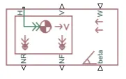
The Vehicle Body block represents a two-axle vehicle body in longitudinal motion. The vehicle can have the same or a different number of wheels on each axle. For example, two wheels on the front axle and one wheel on the rear axle. The vehicle wheels are assumed identical in size. The vehicle can also have a center of gravity (CG) that is at or below the plane of travel.
The block accounts for body mass, aerodynamic drag, road incline, and weight distribution between axles due to acceleration and road profile. Optionally include pitch and suspension dynamics. The vehicle does not move vertically relative to the ground.
The block has an option to include an externally-defined mass and externally-defined inertia. The mass, inertia, and center of gravity of the vehicle body can vary throughout simulation in response to system changes.
- Inport -

Inport blocks link signals from outside a system into the system.
- Outport -

Outport blocks link signals from a system to a destination outside of the system. They can connect signals flowing from a subsystem to other parts of the model. They can also supply external outputs at the top level of a model hierarchy.
- PS Constant -

The PS Constant block generates a physical signal of a constant value. You specify the value and unit of the signal as the Constant parameter.
- Integrator -

- Double-Shoe Brake -

The Double-Shoe Brake block represents a frictional brake with two pivoted rigid shoes that press against a rotating drum to produce a braking action. The rigid shoes sit inside or outside the rotating drum in an opposed configuration. A positive actuating force causes the rigid shoes to press against the rotating drum. Viscous and contact friction between the drum and the rigid shoe surfaces cause the rotating drum to decelerate.
Double-shoe brakes provide high braking torque with small actuator deflections in applications that include motor vehicles and some heavy machinery. The model employs a simple parameterization with readily accessible brake geometry and friction parameters.
You can also enable faulting. When faulting occurs, the belt will exert a user-specified force. Faults can occur at a specified time or due to an external trigger at port T.
- Tire -

The Tire (Simple) block represents a simple, no-slip model of a tire that you parameterize by tire radius.
You can optionally add inertia, stiffness, or damping. These dynamics require additional computation that tends to make models less suitable for real-time simulation.
- Rotational Free End -

The Rotational Free End block represents a mechanical rotational port that rotates freely, without torque.
You can use this block to terminate mechanical rotational ports on other blocks that you want to leave unconnected. This is not necessary because if you leave a conserving port unconnected, the physical network sets all the Through variables at that port to 0. However, terminator blocks improve diagram readability.
You can also use this block to set the initial rotational velocity at a node.
- Gain -

The Gain block multiplies the input by a constant value (gain). The input and the gain can each be a scalar, vector, or matrix.
You specify the value of gain in the Gain parameter. The Multiplication parameter lets you specify element-wise or matrix multiplication. For matrix multiplication, this parameter also lets you indicate the order of the multiplicands.
Gain is converted from doubles to the data type specified in the block mask offline using round-to-nearest and saturation. The input and gain are then multiplied, and the result is converted to the output data type using the specified rounding and overflow modes.
Models:-
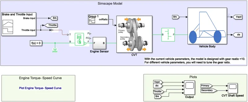
- In this model Brake and Throttle Input are given using a signal builder block. Goto blocks are attached to the signal builder for Brake and Throttle Input signals. Signal Builder is connected to the Engine block of the model through a Simulink-PS connecter.
- Generic Engine a physical block is used as an engine for the model and to observe the Engine RPM signals a subsystem of Engine Sensor is created where an Ideal Rotational Motion Sensor block is used as a sensor and a Scope Block is attached with it to capture the moments of the signal.
- CVT Ratio data are transmitted to the CVT subsystem using a Signal Builder block which is then connected with a Simple Gear block.
- The Simple Gear block is connected to the Vehicle Body which is a Subsystem. A Simple Gear is connected between CVT and Vehicle body for speed deduction.
- Vehicle Body Subsystem has several blocks connected where parameters like mass of the vehicle, Number of wheels, etc are set. One From block which is Brake and two Goto blocks Velocity and Distance is also attached to the Vehicle Body to fetch the respective signals.
- Solver Configuration block and Mechanical Rotational Reference block are also connected for the block.
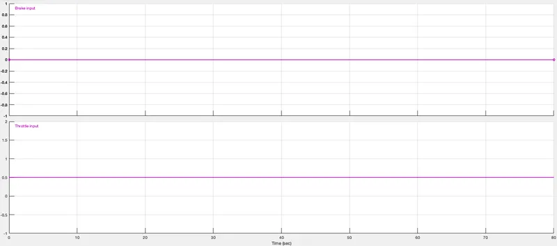
- As seen in the signal builder, Brake Input is 0, and Throttle Input is 0.5 for the model.
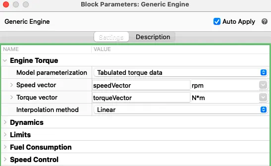
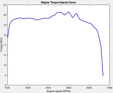
- SpeedVector and TorqueVector data are taken from Engine Torque - Speed Curve.
- Below is the curve that is used for the SpeedVector and TorqueVector data for the model.
- A subsystem is created for the Engine RPM sensor using the Ideal Rotational Motion Sensor. A Scope Block is attached to the physical port W of the RPM sensor to observe its moment, followed by two PMC_port connected to the R port and a Mechanical Rotational Reference to port C, and a PS Terminator is attached to port A.
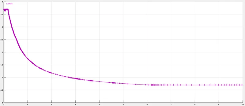
- Below is the CVT Ratio data that is used for the model using a Signal Builder block.
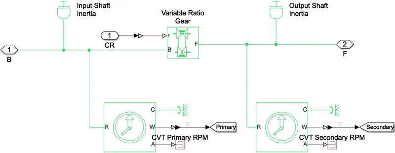
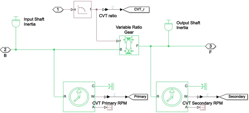
- A Subsystem is created for Continuous Variable Transmission (CVT) using two Inertia blocks Input Shaft Inertia which represents the primary pulley of the vehicle and Output Shaft Inertia represents the secondary pulley of the vehicle and a Variable Ratio Gear block is attached with them.
- Two Ideal Rotational Motion Sensor blocks are also attached to both Inertia block signals and to capture the moment of those signals both the sensors logged with Goto blocks as Primary and secondary.
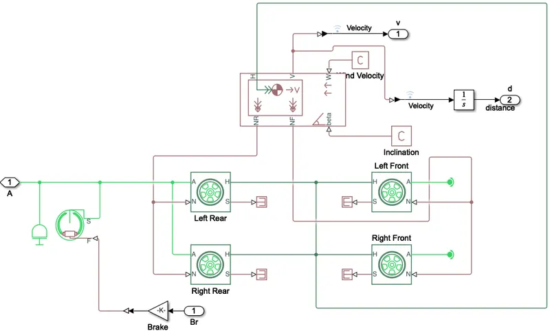
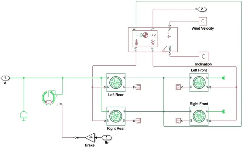
- The vehicle body Subsystem majorly consists of a Vehicle Body block, four tire blocks, and a Double-Shoe Brake block. A PS Constant block as wind velocity is connected to the vehicle body.
- 4 Tire blocks are connected as 2 Rear and 2 Front which are then connected to the Double-Shoe Brake block. The double-Shoe Brake block is directly connected to the secondary pulley of the vehicle. Gain block as Brake is also connected to the f port of the Double-Shoe Brake.
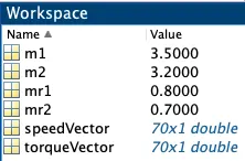
- Below is the Input data which are given through workspace and SpeedVector and TorqueVector are the data from the above curve.
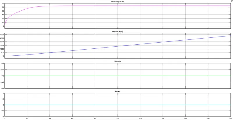
- Below are the Outputs received for the model with a stop time of 200sec.
- In this output, it can be seen that at a constant value of Brake Input 0 and Throttle Input 0.5 Velocity reaches the maximum after 20 sec.
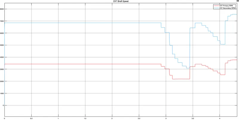
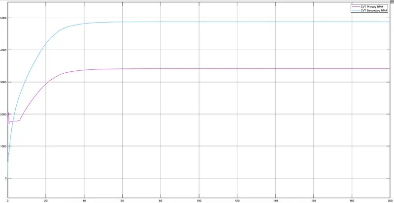
- CVT Secondary RPM can be seen as higher than CVT Primary RPM at a given Brake Input and Throttle Input. Both initially increase till 40sec and then remain constant.
- The Model is similar to the 1st model including Input data. The dashboard is implemented for this model which includes 2 Circular Gauge blocks and 2 Knobs. Input data for Brake and Throttle can be directly changed through Knobs while the model is running.
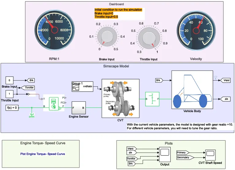
- Circular Gauge blocks are connected to the RPM of the engine and velocity. Deflection for both can be seen when the changes are being made through Brake Input Knob and Throttle Input Knob.
- Two Constant blocks are used in place of Signal Builder. Rest remains the same.
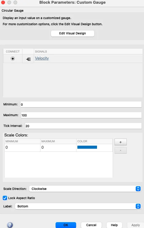
- Through the Circular Gauge parameter, it can be seen that it is connected to the RPM.
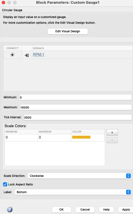
Circular Gauge - Velocity -
- This Circular Gauge is connected to Velocity.
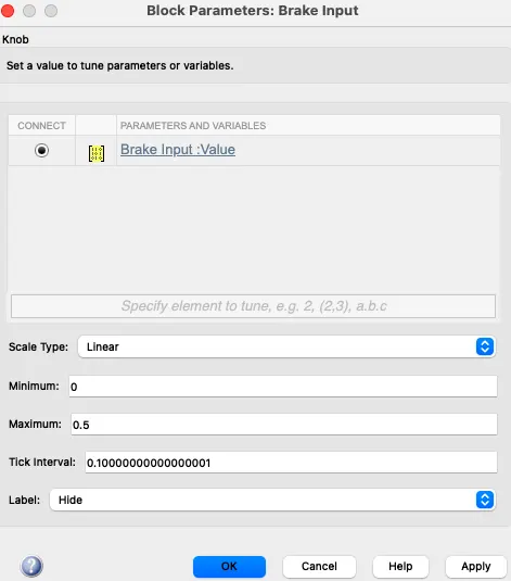
Knob - Brake Input -
- The Knob is connected to the Brake Input.
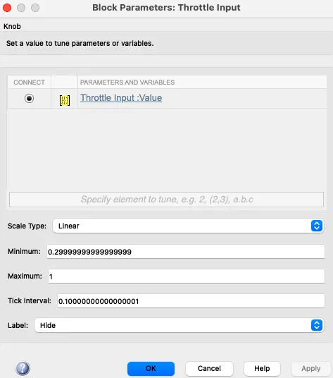
Knob - Throttle Input -
- The Knob is connected to Throttle Input.
Result:-
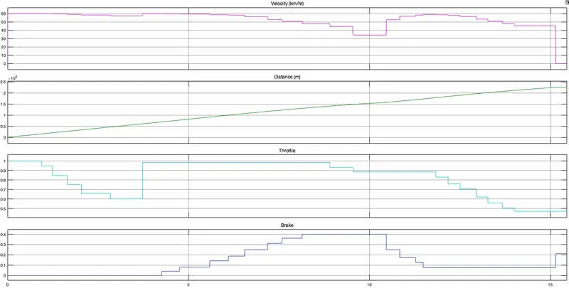
- Changes in the Outputs can be seen with the same Input data as in this model Brake Input and Throttle Input are changed through Knob while the model running. Stop Time for the model used as Infinity as the changes made in the Inputs using Knobs while the model was running.
Output1 -
- Increasing Throttle Input Velocity increases but due to maximum Brake Input, it decreases.
Output2 -
- Similar to the 1st model CVT Secondary RPM is higher than CVT Primary RPM. When Brake Input increases CVT Primary and CVT Secondary RPM decreases and vice versa. Increases when Throttle Input increases.
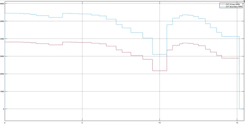
- In this model, some of the Input data like Throttle Input and the CVT ratio data are changed, but the rest remains the same as in previous models.
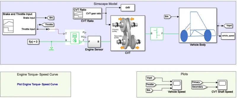
- Brake Input and Throttle Input are given using the Signal Builder block.
- Engine Torque - Speed Curve will be the same as for the previous model.
- 'To Workspace' blocks are used to log the CVT Ratio and Vehicle Speed to the workspace.
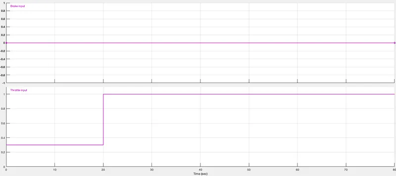
Signal Builder - Throttle & Brake Input -
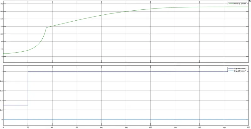
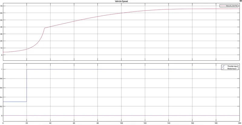
- Compared to the previous models' Brake Input remains constant but Throttle Input changes after 20sec.
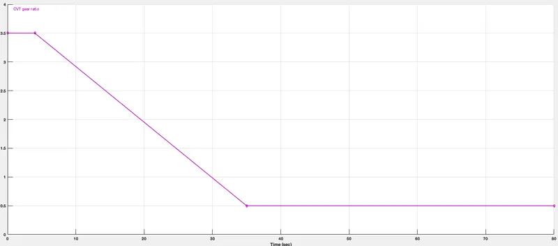
Signal Builder - CVT Gear Ratio -
- Below is the CVT Ratio data used for this model.
Result:-
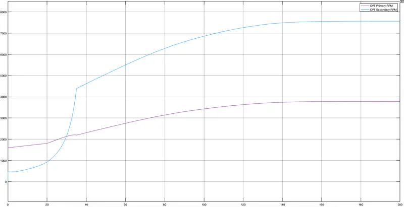
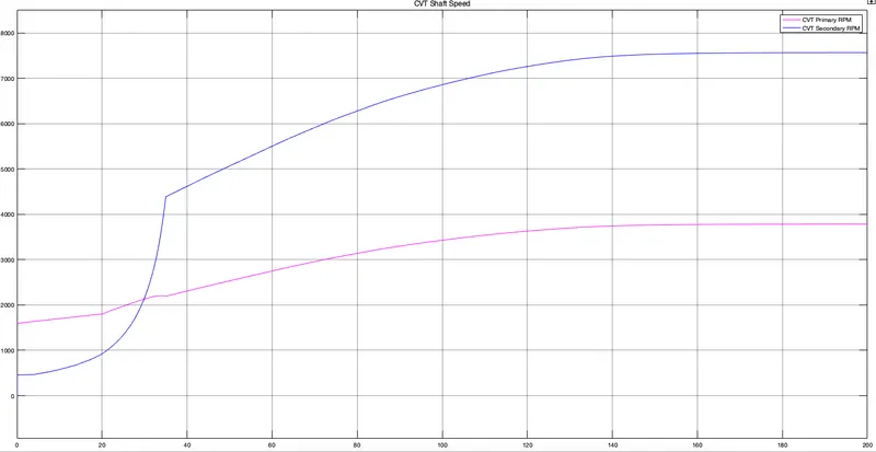
- As the Throttle Input increases after 20sec changes can be seen through the Outputs compared to the previous models. Stop Time used 200sec for the model.
Output1 -
- As per the below scope plots it is seen that when the Throttle Input increases Velocity also increases and reached the maximum.
Output2 -
- CVT Secondary RPM plot can be seen similar to Velocity plot, increasing when the Throttle Input increases. CVT Secondary RPM is higher than the CVT Primary RPM.
Workspace -
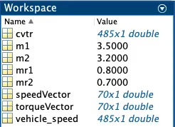
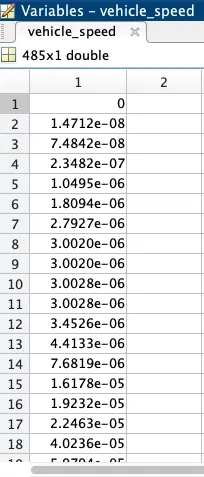
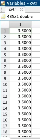
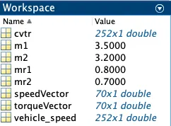
The Primary inputs for the model used remain the same as the previous models. cvtr and vehicle_speed data can be seen in the workspace as To Workspace blocks are used for them.
- The model is almost similar to the previous models apart from a couple of changes like the Lookup Table for the CVT input data.
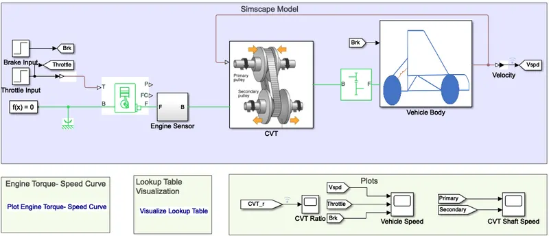
- Step blocks are used for the Brake Input and Throttle Input.
- The signal from Vehicle Body is being reversed to the CVT block making it a closed loop.
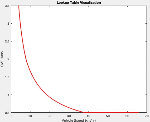
- Engine Torque- Speed Curve remains the same as in previous models. Lookup Table plot is used in this model for CVT data.
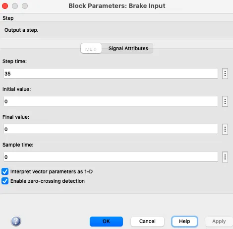
- Brake Input is given in this Step block.
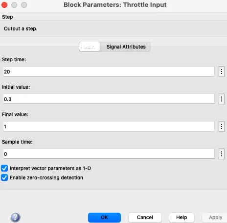
- Throttle Input is given in this Step block.
- Below is the Lookup Table curve used as data in this model.
- Only a change is made in the CVT Subsystem block, a PS lookup table block is used for the CVT data inside the subsystem block compared to the previous model. A Goto block is attached to the lookup table to visualize the data.
- The Vehicle Body remains the same as the other models.
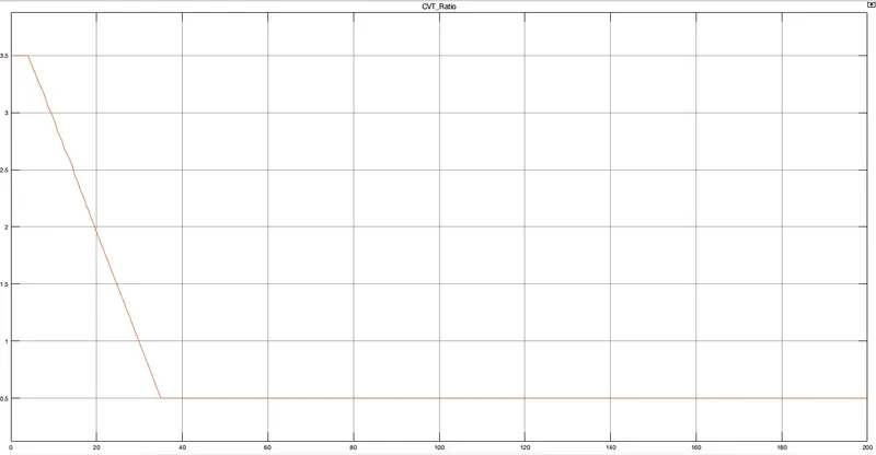
- Below is the CVT Ratio data that is used in the model using the Lookup data table.
- Velocity seems to be resulting the same way compared to the other models where increasing Throttle Input increases the Velocity as well.
- CVT Primary and CVT Secondary RPM responding to the Throttle Input increases when Input is increasing. CVT Secondary RPM is higher than CVT Primary RPM.
- Below are the data received in the workspace.
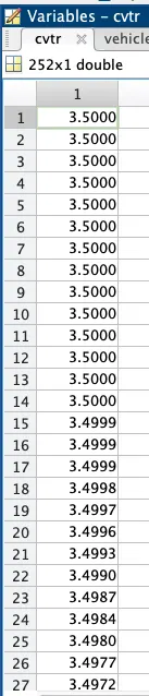
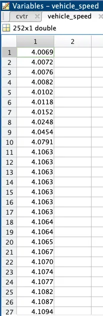
- Similar to the last model only a dashboard block is implemented in this model.
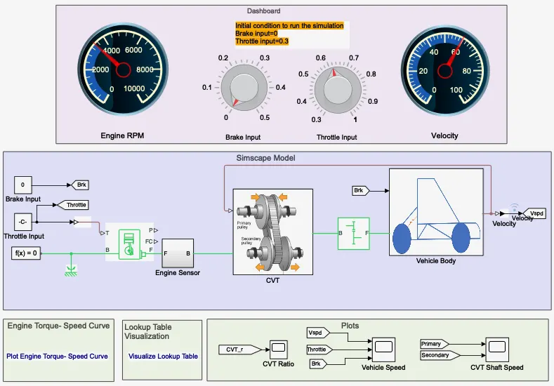
- Compared to the last model, constant blocks are used instead of step blocks for Brake Input and Throttle Input.
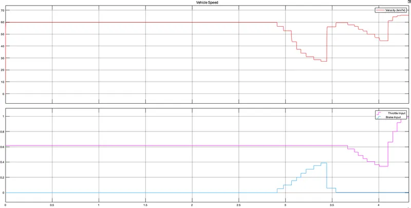
- Changes to the Brake Input and Throttle Input values are made through Knobs while the model is running.
- Below is the CVT Ratio data that is used for the CVT block for this model.
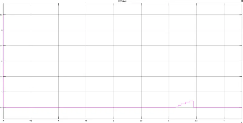
- As per this output when the Throttle Input increases Velocity increases as well and vice versa and when the Brake Input increases Velocity decreases.
- In this Output as well when the Brake Input increases both CVT primary and CVT Secondary RPM decrease and increases when Throttle Input increases.