Project
Carry out a system-level simulation of an all-terrain vehicle.
Download the model from the given link:
https://www.mathworks.com/matlabcentral/fileexchange/70576-baja-all-terrain-vehicle-atv-model
Prepare a technical report explaining the model properties & comments on the results.
Ans-
CVT model_ using signal builder
Components of BAJA ATV are as follows:-
- Vehicle body
- Suspension
- Tire
- Engine
- CVT
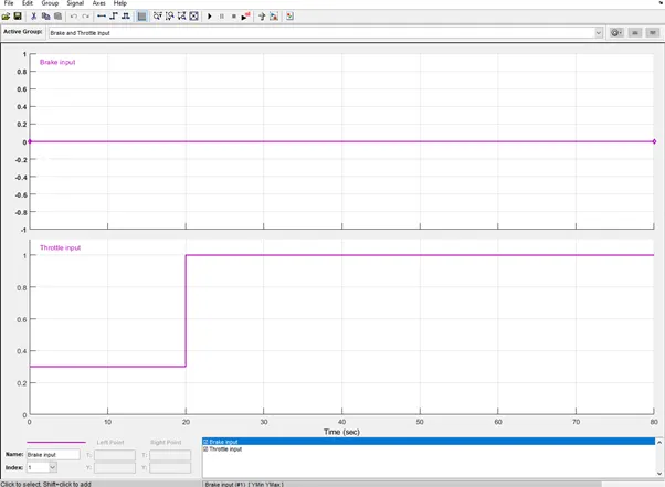
For giving the inputs of break and throttle a signal builder block is been used , the break is been set as constant to zero or not applied for entire simulation and for the throttle the throttle is set as 0.3 from 0 to 20 secs and thereafter the throttle is increased from 0.3 to 1 from 20 to 80 secs.
The signal builder graph for break and throttle is as below:-
After this the outputs are taken from signal builder and the break output is given to GOTO port so that it can be used to connect easily to any other port easily without showing connection lines & the output of throttle is given to the generic engine T port by using Simulink to PS converter as the signal builder is and Simulink model and generic engine is and physical block or simscale block , so we cannot connect it directly so this Simulink to PS converter block is used, Also the throttle output is given to GOTO port for easy connection with other system.
The generic engine is an simple block representing an engine it consists of five ports, port T is input port for throttle input to which the signal of throttle of signal builder is given and Connections F and B are mechanical rotational conserving ports associated with the engine crankshaft and engine block, respectively. Connections P and FC are physical signal output ports through which engine power and fuel consumption rate are reported.
The F port which is an mechanical conversion port of speed of engine crankshaft is given to other subsystem called engine sensor to sense the speed /rpm of engine the B port is connected to the solver configuration and a mechanical reference is also connected to this B port as its and mechanical part , so this solver configuration and mechanical ports are important ports for running simulation successfully.
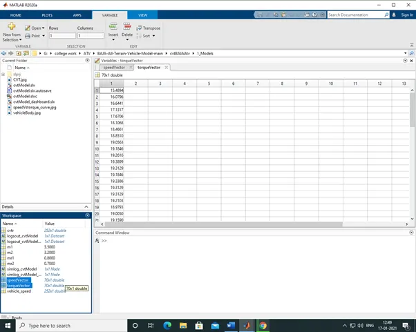
The input parameters for generic engine such as speed vector and torque vector are given by creating an variable in workspace as speedVector and torqueVector
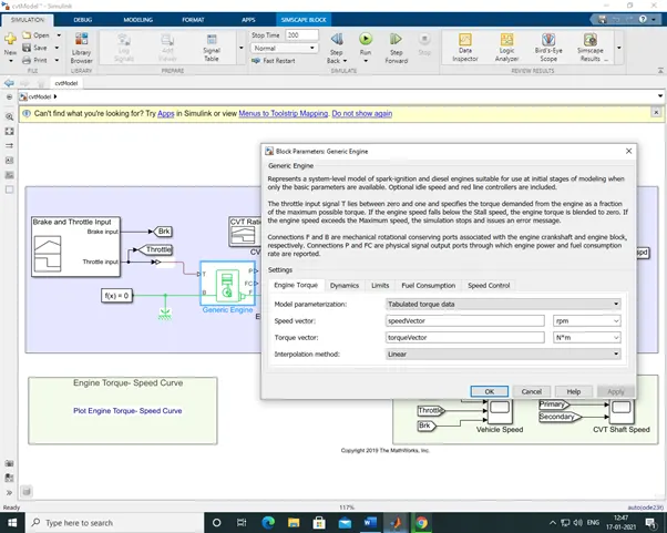
As shown in below fig the variables are created in workspace and the input values are assigned for speed vector and torque vector respectively.
This is the graph which is showing the engine speed torque curve :-
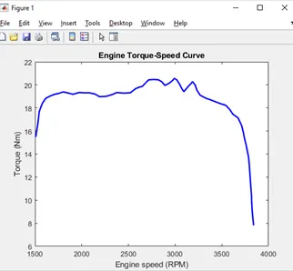
We can se in above graph that the engine speed is starting from 1500 rpm and going upto 3800 rpm and torque is from 6Nm to 22Nm.
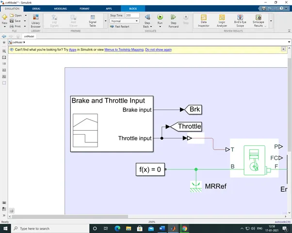
up till now the Simulink model is been modelled as shown above.
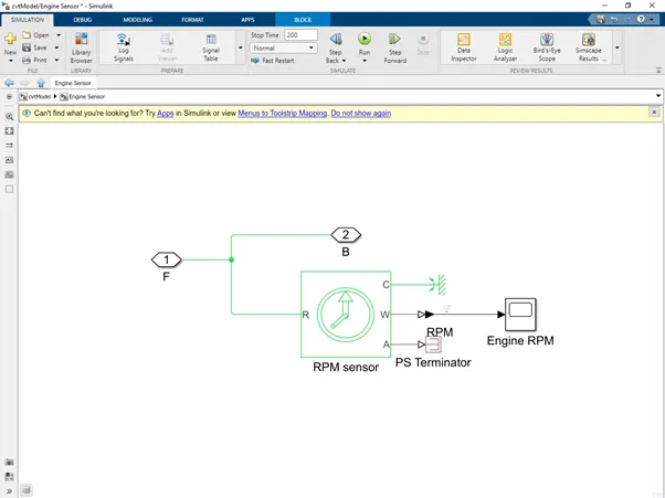
The output of generic engine block F port is connected to ideal rotational motion sensor to R port of it to sense the rpm of crankshaft the ideal rotational motion sensor is nothing but only a sensor to sense the angular velocity, its consists of 5 ports the R port is the input port , Connections R and C are mechanical rotational conserving ports and connections W and A are physical signal output ports for velocity and angular displacement, respectively. The mechanical reference is connected to the C port of ideal rotational motion sensor and W port is connected to the scope to observe the rpm of crankshaft by using the PS-Simulink converter as the ideal rotational motion sensor is an ps block while the scope is an Simulink block , for connecting the W port with scope successfully this block is used. While A port of rotational motion sensor is connected to the PS terminator the use of PS terminator is to terminate physical signal outputs. Unconnected physical signal output ports do not generate warnings, but connection to a PS Terminator can be used to indicate that the signal was not inadvertently left unconnected. After creating this sensor model it’s the created to an subsystem for creating the simplicity in the Simulink model, there are two PMC port in this which enable Physical Modeling Connection Port block for subsystems PMC port 1 & 2 are the connection port for the subsystem.
The subsystem is named as engine sensor and if the subsystem is opened it looks like below as shown in fig-
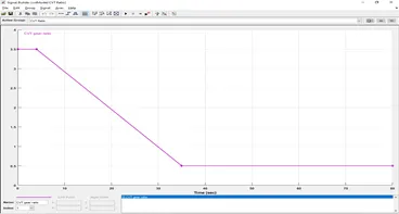
A one more signal builder block is used for creating CVT gear ratio at start the gear ratio is 3.5 from 0 to 5 sec and thereafter its decreasing from 3.5 to 0.5 from 5 sec to 35 secs and thereafter the gear ratio is constant from 35 sec to 80 secs.
The signal builder graph looks like below shown in fig after creating the required signal :-
The signal of CVT gear ratio from signal builder is given to the subsystem CVT by using inport block to variable ratio transmission block, the variable ratio transmission Represents a variable ratio gearbox such as implemented by mechanical belt CVT, electric, or hydraulic transmissions. The physical signal input r defines the ratio of input to output angular shaft velocities.
Connections B (base) and F (follower) are mechanical rotational conserving ports.
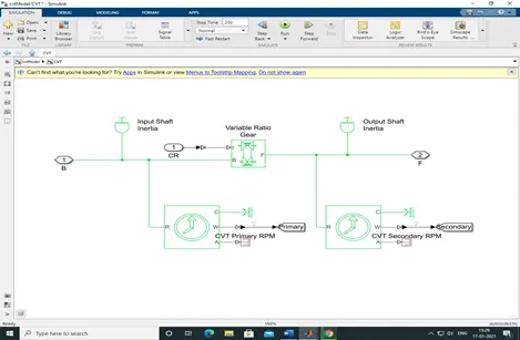
The output of generic engine F port is connected to B port of variable ratio transmission through engine sensor subsystem output port B , to the input B port of variable ratio transmission a ideal rotational motion sensor and inertia block are connected to sense the angular motion and to provide a inertia to the base of variable ratio transmission , the R port of ideal rotational motion sensor is connected to the base of variable ratio transmission B port and C, W & A port of ideal rotational motion sensor are connected to the mechanical reference block, scope with the help of PS-simulink converter block and PS terminator block respectively.
The other port of variable ratio transmission block i.e- F port (follower) is taken out , to this also a ideal rotational motion sensor is connected to sense the angular motion of sensor , this is connected in similar manner as the previous rotational sensor was connected to the base of variable ratio transmission, also for this port the inertia block is connected to provide inertia . the inertia block doesn’t have any operation related to this system only the help in configuring the system.
The angular motion that we have sensed for the base and follower are named as primary and secondary rpm respectively. The output of this both the rotational sensors are connected to the GOTO port (W was the output port of this sensors)
The subsystem of CVT looks like follow:-
The follower output of variable ratio transmission (F port) is taken out from the subsystem with the help of PMC port and connected to the simple gear block B port or base port the ratio of base to the follower of simple gear is set as 12 , the simple gear block is connected only because to reduce the rpm of secondary pulley of CVT
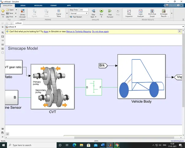
Now we have to modal a vehicle body or vehicle body subsystem:-
For this we will be using –
- Vehicle body block
- Tire block (4 blocks of tire)
- Double shoe brake
This 3 are some important blocks for modelling a vehicle body subsystem.
The subsystem of vehicle body looks like below-
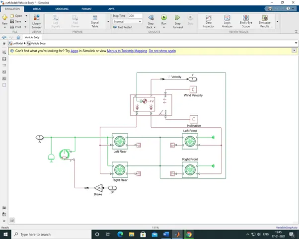
The vehicle body as 6 ports ,
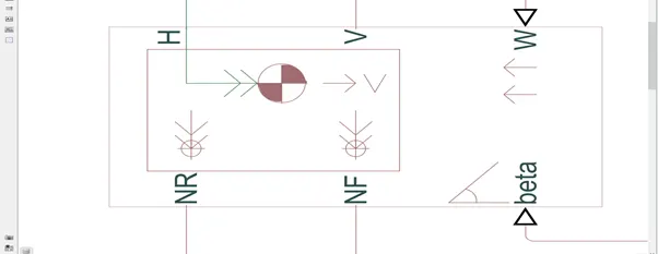
connection H is the mechanical translational conserving port associated with the horizontal motion of the vehicle body. The resulting traction motion developed by tires should be connected to this port.
Connections V, NF, and NR are physical signal output ports for vehicle velocity and front and rear normal wheel forces, respectively.
Connections W and beta are physical signal input ports corresponding to headwind speed and road inclination angle, respectively.
The vehicle body look like this-
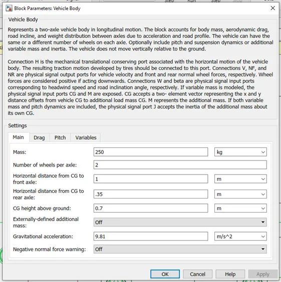
The parameter for vehicle body are set as follows-
The NR port of vehicle body is the rear axle port and we have set the number of wheels per axle as 2 so we will connect 2 tires to this NR port , this NR port will be connected to the N port of tire as N port is the physical signal input port. In similar manner the NF port is connected to the 2 tire blocks in similar manner.
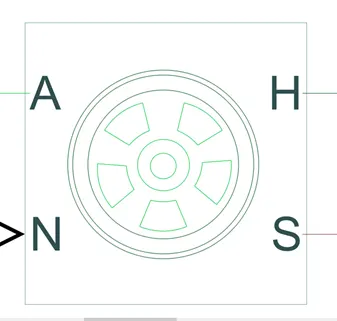
The tire block as 4 number of ports as A, N, H & S
Connection A is the mechanical rotational conserving port for the wheel axle.
Connection H is the mechanical translational conserving port for the wheel hub through which the thrust developed by the tire is applied to the vehicle.
Connection N is a physical signal input port that applies the normal force acting on the tire. The force is considered positive if it acts downwards.
Connection S is a physical signal output port that reports the tire slip.
The tire block looks like follow-
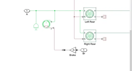
To both the rear tires the output of simple gear follower is connected to the A port of both the rear tire i.e left rear and right rear . there will be no direct drive from follower of simple gear to the front axle or wheels. Also the inertia and double shoe brake are connected in between the F port simple gear and A port of tire block.
The double shoe brake has 2 ports-
Connection S is a conserving rotational terminal associated with the drum shaft.
Connection F is a physical signal port representing the force input to the actuator. Positive force creates friction torque that resists shaft rotation.
The input of brake are taken from signal builder of brake and throttle input to the brake shoe F port with the help of from block and then sent inside the subsystem of vehicle body with the help of inport block. Then this signal from inport block are given to the gain block which will multiply the input force , to connect this gain block with the F port of double shoe brake a Simulink to PS converter block is used.
The connection will look like this-
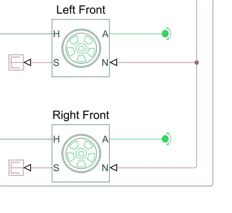
The A ports of front tire i.e left front and right front will be connected to the rotational free end block.
The connection of A port of front wheels will like this-
The input parameters for all the 4 tires are set as default , no any changes are made in parameters of tire.
The H port of left rear and left front are connected with each other as H port is the mechanical translational conserving port
While the H port of right rear and front front are connected with each other as H port is the mechanical translational conserving port, and S port of all 4 tires are connected to PS terminator individually.
A PS constant blocks are used to connecte the W & beta ports of vehicle body. The PS constant block are set as 0 for both W & beta input values.
The V port of vehicle body block is the output port for vehicle velocity as we have discussed earlier so this block connection is taken out of subsystem with the help of output port and after this its connected to GOTO port so that it can be connected to the scope for viewing results without showing the connection lines. This GOTO port is named or tag as Vsped.
Now all the GOTO ports of throttle , brake , Vehicle speed , primary and secondary are connected to the scope with the help of from block to the scope,
There are two scops at the end for viewing results , for first scope the outputs or results of vehicle speed , throttle and brake are displayed and in the second scope the graph of primary and secondary rpm of CVT are is been observed.
The first scope is been named as Vehicle speed and the second scope is named as CVT shaft speed .
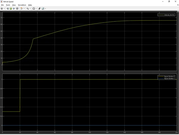
The result of vehicle speed scope are as shown in below fig-
And the results of CVT shaft speed are as shown in below fig-
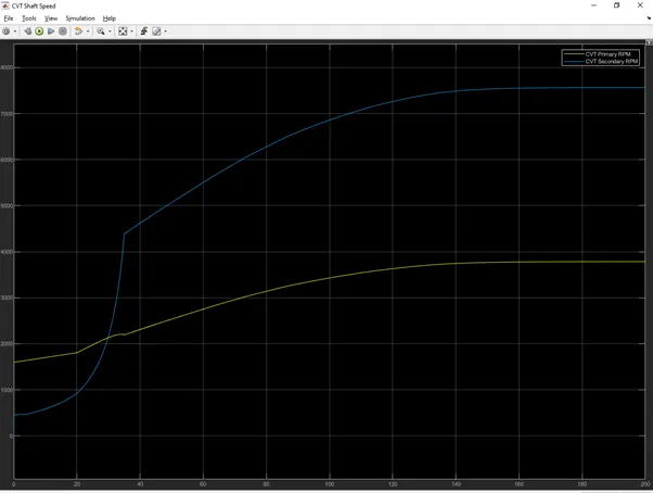
From this both the graph or results obtain from the 2 scope we can conclude that-
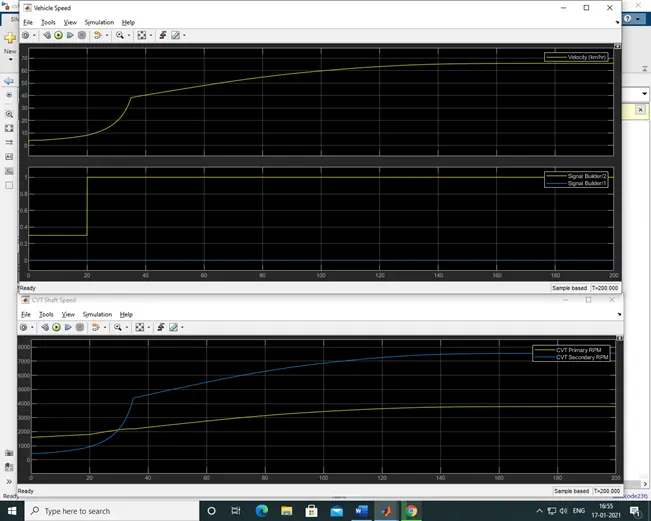
As the throttle is increased the rpm of engine is increasing which leads to increase in speed of primary shaft of CVT gear box further the CVT gear is changed which leads to change in the speed of secondary shaft of CVT and as mention in signal builder block of CVT ratio the ratio will change and the secondary shaft of CVT will be overdriven and the final speed of vehicle will increase.
If we will check the scope or compare it with each other then we see that as secondary shaft ratio is increasing from 0.5 secs to 35 secs then at the same time the vehicle speed is increased.
In below fig the results of both the scope are placed or arranged one below the other so that it can be visualized easily.
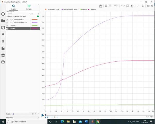
The below fig shows the results from data inspector-
In this results the engine rpm is tracing the primary shaft rpm as the rpm of both are same and there is no any reduction or gain after engine shaft and primary shaft of CVT and as secondary shaft rpm is increasing the velocity of vehicle is increasing.
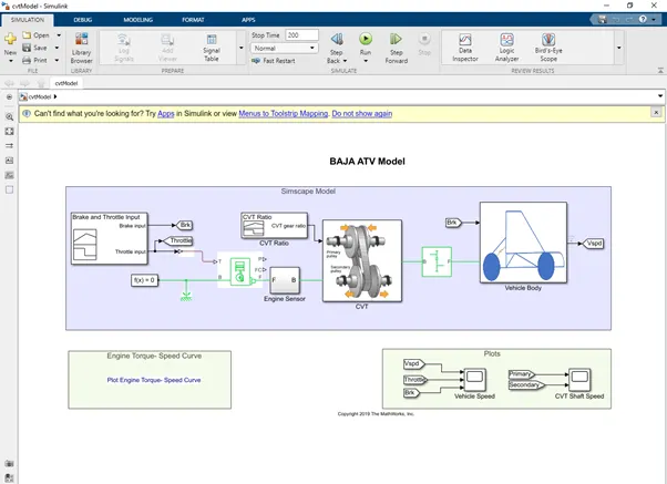
The final model of ATV will look like follow-
*********************************************************************************************************************************************************************************************************************************************************************************************************************************************************************************************************************************************************************************
BAJA ATV MODEL
WITH LOOK UP TABLE
As we have seen in the previous model of CVT we had used the signal builder block for providing the input signals for brake and throttle, in this model instead of signal builder we are giving the input signals of brake and throttle by using step block.
The step block look like this-
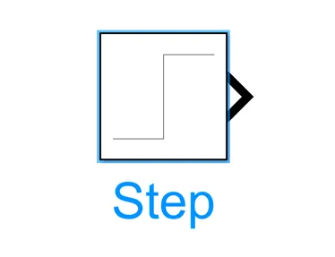
The Step block provides a step between two definable levels at a specified time.
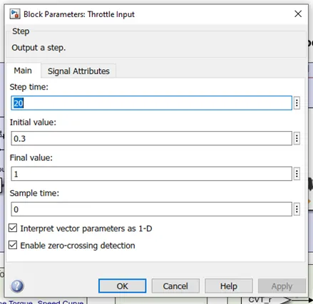
Here 2 step blocks are been used for throttle and brake respectively .the parameter for throttle is set as follows –
- Step time -20
- Initial value -0.3
- Final value -1
- Sample time -0
Throttle input parameter-
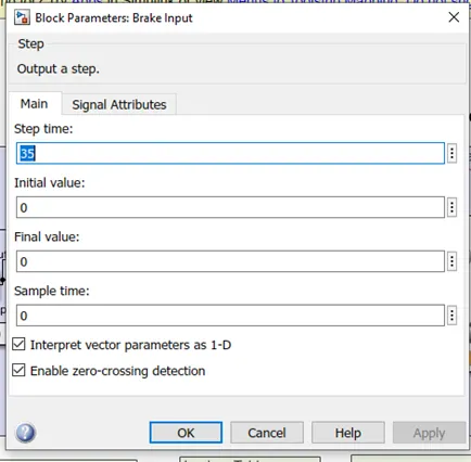
The brake input parameter are as follows-
- Step time -35
- Initial value -0
- Final value - 0
- Sample time -0
Brake input parameter-
After this the outputs are taken from both the step block respectively and the break output is given to GOTO port so that it can be used to connect easily to any other port easily without showing connection lines & the output of throttle is given to the generic engine T port by using Simulink to PS converter as the signal builder is and Simulink model and generic engine is and physical block or simscale block , so we cannot connect it directly so this Simulink to PS converter block is used, Also the throttle output is given to GOTO port for easy connection with other system.
The generic engine is an simple block representing an engine it consists of five ports, port T is input port for throttle input to which the signal of throttle of signal builder is given and Connections F and B are mechanical rotational conserving ports associated with the engine crankshaft and engine block, respectively. Connections P and FC are physical signal output ports through which engine power and fuel consumption rate are reported.
The F port which is an mechanical conversion port of speed of engine crankshaft is given to other subsystem called engine sensor to sense the speed /rpm of engine the B port is connected to the solver configuration and a mechanical reference is also connected to this B port as its and mechanical part , so this solver configuration and mechanical ports are important ports for running simulation successfully.
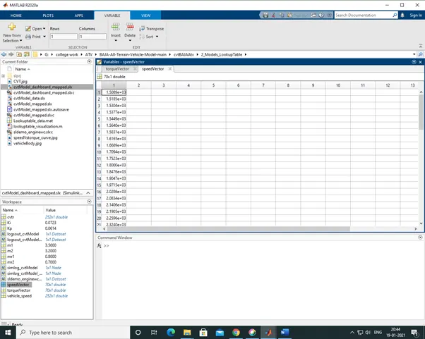
The input parameters for generic engine such as speed vector and torque vector are given by creating an variable in workspace as speedVector and torqueVector
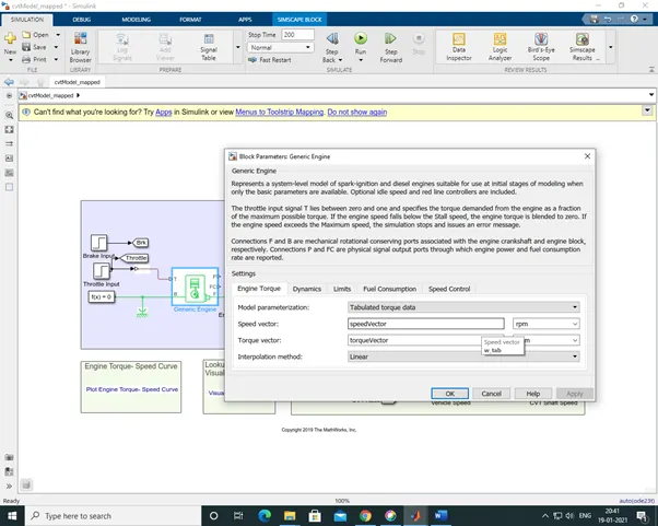
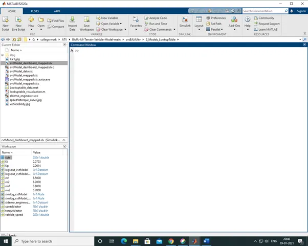
As shown in below fig the variables are created in workspace and the input values are assigned for speed vector and torque vector respectively.
This is the graph which is showing the engine speed torque curve :-
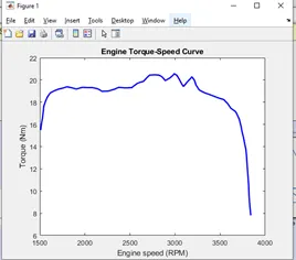
We can se in above graph that the engine speed is starting from 1500 rpm and going upto 3800 rpm and torque is from 6Nm to 22Nm.
This is how the blocks are connected as per this condition-
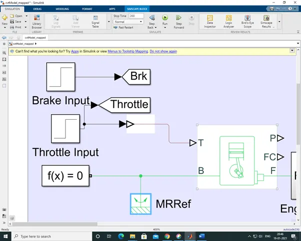
The output of generic engine block F port is connected to ideal rotational motion sensor to R port of it to sense the rpm of crankshaft the ideal rotational motion sensor is nothing but only a sensor to sense the angular velocity, its consists of 5 ports the R port is the input port , Connections R and C are mechanical rotational conserving ports and connections W and A are physical signal output ports for velocity and angular displacement, respectively. The mechanical reference is connected to the C port of ideal rotational motion sensor and W port is connected to the scope to observe the rpm of crankshaft by using the PS-Simulink converter as the ideal rotational motion sensor is an ps block while the scope is an Simulink block , for connecting the W port with scope successfully this block is used. While A port of rotational motion sensor is connected to the PS terminator the use of PS terminator is to terminate physical signal outputs. Unconnected physical signal output ports do not generate warnings, but connection to a PS Terminator can be used to indicate that the signal was not inadvertently left unconnected. After creating this sensor model it’s the created to an subsystem for creating the simplicity in the Simulink model, there are two PMC port in this which enable Physical Modeling Connection Port block for subsystems PMC port 1 & 2 are the connection port for the subsystem.
The subsystem is named as engine sensor and if the subsystem is opened it looks like below as shown in fig-
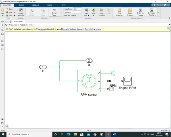
The subsystem for engine sensor is been modelled now after sensing the engine rpm thr F port of the generic engine block is given to the variable ratio transmission block B port , , the variable ratio transmission Represents a variable ratio gearbox such as implemented by mechanical belt CVT, electric, or hydraulic transmissions. The physical signal input r defines the ratio of input to output angular shaft velocities.
Connections B (base) and F (follower) are mechanical rotational conserving ports.
The output of generic engine F port is connected to B port of variable ratio transmission through engine sensor subsystem output port B , to the input B port of variable ratio transmission a ideal rotational motion sensor and inertia block are connected to sense the angular motion and to provide a inertia to the base of variable ratio transmission , the R port of ideal rotational motion sensor is connected to the base of variable ratio transmission B port and C, W & A port of ideal rotational motion sensor are connected to the mechanical reference block, scope with the help of PS-simulink converter block and PS terminator block respectively.
The other port of variable ratio transmission block i.e- F port (follower) is taken out , to this also a ideal rotational motion sensor is connected to sense the angular motion of sensor , this is connected in similar manner as the previous rotational sensor was connected to the base of variable ratio transmission, also for this port the inertia block is connected to provide inertia . the inertia block doesn’t have any operation related to this system only the help in configuring the system.
Here the 2 variables are created that are m1 & m2 for the values of inertia of base and follower of variable ratio transmission block respectively. The values of m1 & m2 are set as 3.5 and 3.2 respectively.
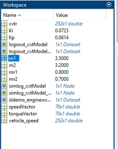
The angular motion that we have sensed for the base and follower are named as primary and secondary rpm respectively. The output of this both the rotational sensors are connected to the GOTO port (W was the output port of this sensors)
The subsystem of CVT will like this-
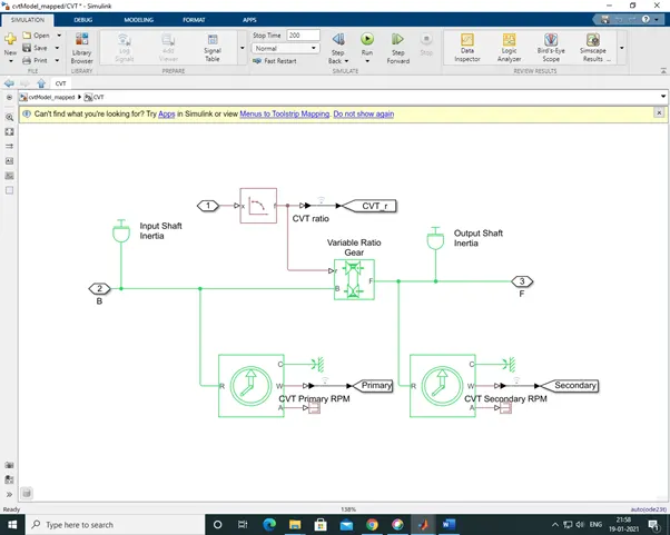
In previous model of CVT we used a signal builder block which gave the input signal to the R port of variable ratio transmission block here instead of signal builder block we are using a look up table block ,
The PS Lookup Table block computes an approximation to some function f=f(x) given data vectors x and f. Both the input and the output are physical signals.
The length of the x and f data vectors provided to this block must match. Also, the x data vector must be strictly monotonic, either increasing or decreasing.
Plotting a lookup table lets you visualize the data before simulating the model, to make sure that the table is correct. The plot reflects tabulated data specified for the block, as well as the selected interpolation and extrapolation options.
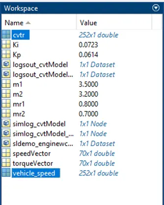
For setting the look up table there is need to provide the values for table grid values and table values the values are entered in this block by creating the variables for it the variable which is created for values of table grid is named as vehicle speed and this values which are specified for vehicle speed in the workspace is further divided by 3.6
And the variable which is created for table value is named as cvtr.
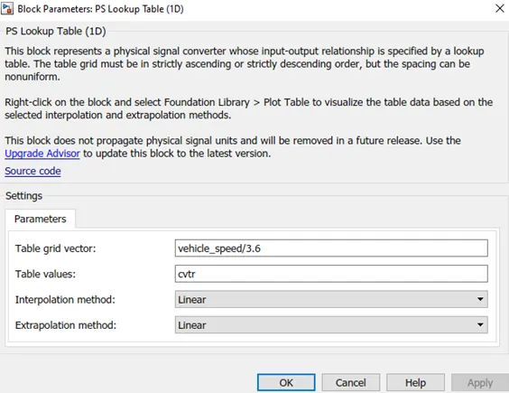
The variable which are created for vehicle speed and cvtr in workspace window are like this-
The look up table will look like follow-
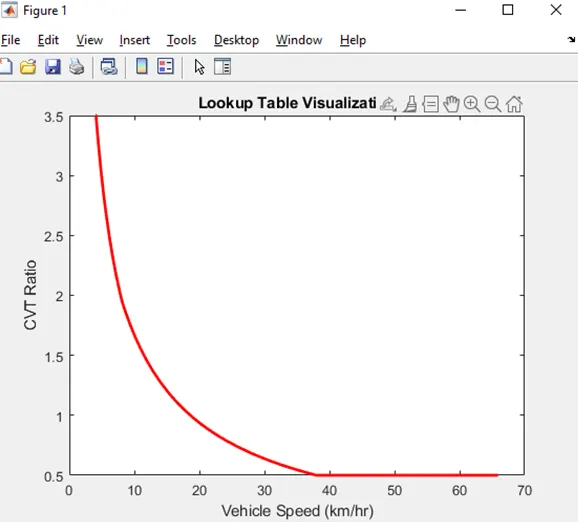
The look up table will compare the speed of vehicle with the help of the values specified in look up table and as per it the ratio of cvt will be set .
The above fig shown the visual look up table graph in which manner the cvt ratio will change with respect to speed.
the output port V of vehicle body table is connected with the x port of look up table which is input port , further we are going to see the vehicle body block in that we will discuss in brief about the block. And the F port of look up table is connected with the input R port of variable ratio transmission block along with this the output port F of look up table is given to the goto port which will allow us to see or connect with the scope out of the subsystem. Here for connecting the F port of look up table with the goto port we require a PS – Simulink converter block as this both the block are from different libraries.
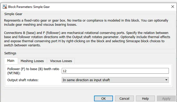
The follower output of variable ratio transmission (F port) is taken out from the subsystem with the help of PMC port and connected to the simple gear block B port or base port the ratio of base to the follower of simple gear is set as 12 , the simple gear block is connected only because to reduce the rpm of secondary pulley of CVT
The parameter for simple gear are set as shown in below fig-
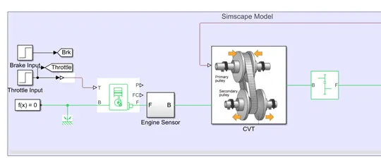
Now the model is been modelled upto the simple gear block which in real life model is differential ,further we have to give this signal to the final drive that is wheels of the vehicle body , for that we have to model further the model of vehicle body
The model of Simulink will look like follow till now-
Now we have to modal a vehicle body or vehicle body subsystem:-
For this we will be using –
- Vehicle body block
- Tire block (4 blocks of tire)
- Double shoe brake
This 3 are some important blocks for modelling a vehicle body subsystem.
The subsystem of vehicle body looks like below-
The vehicle body as 6 ports ,
connection H is the mechanical translational conserving port associated with the horizontal motion of the vehicle body. The resulting traction motion developed by tires should be connected to this port.
Connections V, NF, and NR are physical signal output ports for vehicle velocity and front and rear normal wheel forces, respectively.
Connections W and beta are physical signal input ports corresponding to headwind speed and road inclination angle, respectively.
The vehicle body look like this-
The parameter for vehicle body are set as follows-
The NR port of vehicle body is the rear axle port and we have set the number of wheels per axle as 2 so we will connect 2 tires to this NR port , this NR port will be connected to the N port of tire as N port is the physical signal input port. In similar manner the NF port is connected to the 2 tire blocks in similar manner.
The tire block as 4 number of ports as A, N, H & S
Connection A is the mechanical rotational conserving port for the wheel axle.
Connection H is the mechanical translational conserving port for the wheel hub through which the thrust developed by the tire is applied to the vehicle.
Connection N is a physical signal input port that applies the normal force acting on the tire. The force is considered positive if it acts downwards.
Connection S is a physical signal output port that reports the tire slip.
The tire block looks like follow-
To both the rear tires the output of simple gear follower is connected to the A port of both the rear tire i.e left rear and right rear . there will be no direct drive from follower of simple gear to the front axle or wheels. Also the inertia and double shoe brake are connected in between the F port simple gear and A port of tire block.
The double shoe brake has 2 ports-
Connection S is a conserving rotational terminal associated with the drum shaft.
Connection F is a physical signal port representing the force input to the actuator. Positive force creates friction torque that resists shaft rotation.
The input of brake are taken from step block and given to input of the brake shoe F port with the help of from block and then sent inside the subsystem of vehicle body with the help of inport block. Then this signal from inport block are given to the gain block which will multiply the input force , to connect this gain block with the F port of double shoe brake a Simulink to PS converter block is used.
The connection will look like this-
The A ports of front tire i.e left front and right front will be connected to the rotational free end block.
The connection of A port of front wheels will like this-
The input parameters for all the 4 tires are set as default , no any changes are made in parameters of tire.
The H port of left rear and left front are connected with each other as H port is the mechanical translational conserving port
While the H port of right rear and front front are connected with each other as H port is the mechanical translational conserving port, and S port of all 4 tires are connected to PS terminator individually.
A PS constant blocks are used to connecte the W & beta ports of vehicle body. The PS constant block are set as 0 for both W & beta input values.
The V port of vehicle body block is the output port for vehicle velocity as we have discussed earlier so this block connection is taken out of subsystem with the help of output port and along with this the signal of velocity is given to the look up table input F port , as we have discussed earlier while describing the look up table , so that now the close loop is been formed between the model. The signal of V port of vehicle body which we have taken out of the subsystem is connected to GOTO port so that it can be connected to the scope for viewing results without showing the connection lines. This GOTO port is named or tag as Vsped.
Now all the GOTO ports of throttle , brake , Vehicle speed , cvtr, primary and secondary are connected to the scope with the help of from block to the scope,
There are three scops at the end for viewing results , for first scope the outputs or results of vehicle speed , throttle and brake are displayed and in the second scope the graph of primary and secondary rpm of CVT are is been observed. And in the third scope the result/graph of cvt is observed.
The first scope is been named as Vehicle speed and the second scope is named as CVT shaft speed and the third scope is named as CVT ratio .
The result of vehicle speed scope are as shown in below fig-
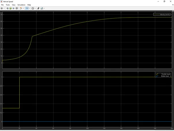
From this scope of vehicle speed we see that the throttle is 0.3 for starting of simulation that is from 0 to 20 sec and after that the throttle is increased from 0.3 to 1 from 20 sec till enf of simulation and the brake value is 0 throughout the simulation as we have mention this parameters in stem block of throttle and brake.
From this inputs of throttle and brake the we see that the vehicle speed is behaving as per it , there is gradual speed of 4km/hr and increasing slowly but when the throttle is applied the speed of vehicle is increasing in a vary rapid manner and when the desired value of throttle is obtained of 1 after that the speed of vehicle is again increasing in gradual manner the top speed of atv which is reached is about 65.9km/hr.
The result of the second scope are as shown in below fig:-
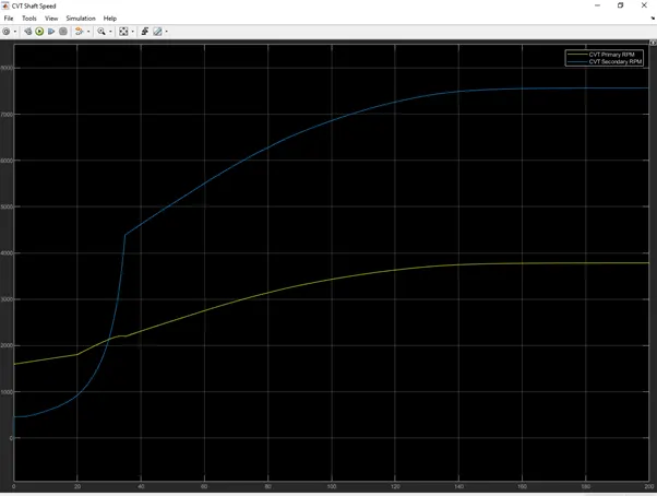
The yellow line in the graph represents the primary shaft rpm and the blue line indicate the rpm of secondary rpm. The gear ratio is changing the ratio depending upon the speed .
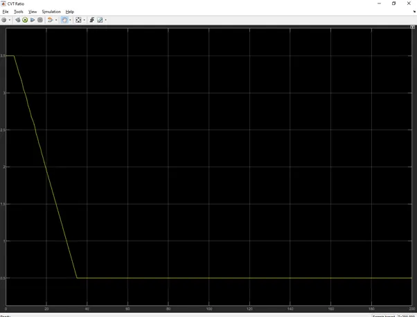
The results of the third scope are as shown in below fig-
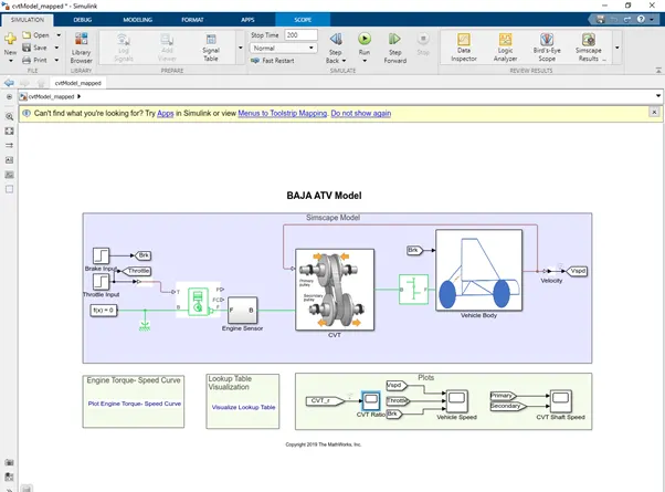
The final model of BAJA ATV with LOOK UP TABLE look like below-
*********************************************************************************************************************************************************************************************************************************************************************************************************************************************************************************************************************************************************************************
BAJA ATV MODEL CVT DATA MODEL:-
There is not much difference between the model of BAJA ATV model using signal builder block and this model of BAJA ATV MODEL CVT DATA MODEL here only one additional block is used of from TO WORKSPACE to save the data of cvt gear box in workspace window by creating the variable name of it.
Here the variable will be created in the workspace window as we have assigned for it
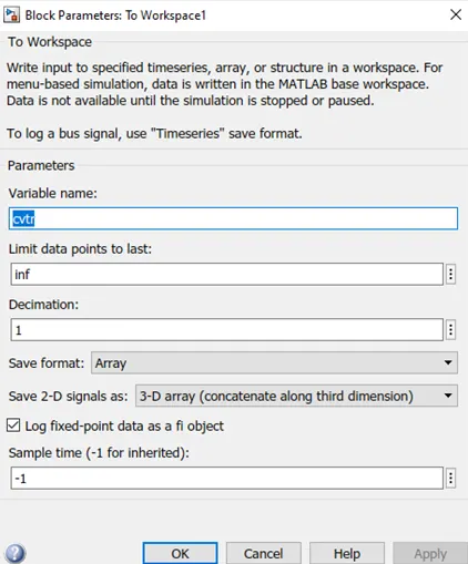
Here the variable name is given as cvtr , so this variable will be created in workspace window.it look like this in workspace-
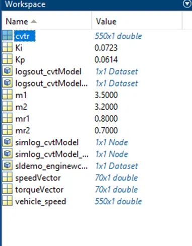
Rest of the system is same____
Components of BAJA ATV are as follows:-
- Vehicle body
- Suspension
- Tire
- Engine
- CVT
For giving the inputs of break and throttle a signal builder block is been used , the break is been set as constant to zero or not applied for entire simulation and for the throttle the throttle is set as 0.3 from 0 to 20 secs and thereafter the throttle is increased from 0.3 to 1 from 20 to 80 secs.
The signal builder graph for break and throttle is as below:-
After this the outputs are taken from signal builder and the break output is given to GOTO port so that it can be used to connect easily to any other port easily without showing connection lines & the output of throttle is given to the generic engine T port by using Simulink to PS converter as the signal builder is and Simulink model and generic engine is and physical block or simscale block , so we cannot connect it directly so this Simulink to PS converter block is used, Also the throttle output is given to GOTO port for easy connection with other system.
The generic engine is an simple block representing an engine it consists of five ports, port T is input port for throttle input to which the signal of throttle of signal builder is given and Connections F and B are mechanical rotational conserving ports associated with the engine crankshaft and engine block, respectively. Connections P and FC are physical signal output ports through which engine power and fuel consumption rate are reported.
The F port which is an mechanical conversion port of speed of engine crankshaft is given to other subsystem called engine sensor to sense the speed /rpm of engine the B port is connected to the solver configuration and a mechanical reference is also connected to this B port as its and mechanical part , so this solver configuration and mechanical ports are important ports for running simulation successfully.
The input parameters for generic engine such as speed vector and torque vector are given by creating an variable in workspace as speedVector and torqueVector
As shown in below fig the variables are created in workspace and the input values are assigned for speed vector and torque vector respectively.
This is the graph which is showing the engine speed torque curve :-
We can se in above graph that the engine speed is starting from 1500 rpm and going upto 3800 rpm and torque is from 6Nm to 22Nm.
up till now the Simulink model is been modelled as shown above.
The output of generic engine block F port is connected to ideal rotational motion sensor to R port of it to sense the rpm of crankshaft the ideal rotational motion sensor is nothing but only a sensor to sense the angular velocity, its consists of 5 ports the R port is the input port , Connections R and C are mechanical rotational conserving ports and connections W and A are physical signal output ports for velocity and angular displacement, respectively. The mechanical reference is connected to the C port of ideal rotational motion sensor and W port is connected to the scope to observe the rpm of crankshaft by using the PS-Simulink converter as the ideal rotational motion sensor is an ps block while the scope is an Simulink block , for connecting the W port with scope successfully this block is used. While A port of rotational motion sensor is connected to the PS terminator the use of PS terminator is to terminate physical signal outputs. Unconnected physical signal output ports do not generate warnings, but connection to a PS Terminator can be used to indicate that the signal was not inadvertently left unconnected. After creating this sensor model it’s the created to an subsystem for creating the simplicity in the Simulink model, there are two PMC port in this which enable Physical Modeling Connection Port block for subsystems PMC port 1 & 2 are the connection port for the subsystem.
The subsystem is named as engine sensor and if the subsystem is opened it looks like below as shown in fig-
A one more signal builder block is used for creating CVT gear ratio at start the gear ratio is 3.5 from 0 to 5 sec and thereafter its decreasing from 3.5 to 0.5 from 5 sec to 35 secs and thereafter the gear ratio is constant from 35 sec to 80 secs.
The signal builder graph looks like below shown in fig after creating the required signal :-
The signal of CVT gear ratio from signal builder is given to the subsystem CVT by using inport block to variable ratio transmission block, the variable ratio transmission Represents a variable ratio gearbox such as implemented by mechanical belt CVT, electric, or hydraulic transmissions. The physical signal input r defines the ratio of input to output angular shaft velocities.
Connections B (base) and F (follower) are mechanical rotational conserving ports.
The output of generic engine F port is connected to B port of variable ratio transmission through engine sensor subsystem output port B , to the input B port of variable ratio transmission a ideal rotational motion sensor and inertia block are connected to sense the angular motion and to provide a inertia to the base of variable ratio transmission , the R port of ideal rotational motion sensor is connected to the base of variable ratio transmission B port and C, W & A port of ideal rotational motion sensor are connected to the mechanical reference block, scope with the help of PS-simulink converter block and PS terminator block respectively.
The other port of variable ratio transmission block i.e- F port (follower) is taken out , to this also a ideal rotational motion sensor is connected to sense the angular motion of sensor , this is connected in similar manner as the previous rotational sensor was connected to the base of variable ratio transmission, also for this port the inertia block is connected to provide inertia . the inertia block doesn’t have any operation related to this system only the help in configuring the system.
The angular motion that we have sensed for the base and follower are named as primary and secondary rpm respectively. The output of this both the rotational sensors are connected to the GOTO port (W was the output port of this sensors)
The subsystem of CVT looks like follow:-
The follower output of variable ratio transmission (F port) is taken out from the subsystem with the help of PMC port and connected to the simple gear block B port or base port the ratio of base to the follower of simple gear is set as 12 , the simple gear block is connected only because to reduce the rpm of secondary pulley of CVT
Now we have to modal a vehicle body or vehicle body subsystem:-
For this we will be using –
- Vehicle body block
- Tire block (4 blocks of tire)
- Double shoe brake
This 3 are some important blocks for modelling a vehicle body subsystem.
The subsystem of vehicle body looks like below-
The vehicle body as 6 ports ,
connection H is the mechanical translational conserving port associated with the horizontal motion of the vehicle body. The resulting traction motion developed by tires should be connected to this port.
Connections V, NF, and NR are physical signal output ports for vehicle velocity and front and rear normal wheel forces, respectively.
Connections W and beta are physical signal input ports corresponding to headwind speed and road inclination angle, respectively.
The vehicle body look like this-
The parameter for vehicle body are set as follows-
The NR port of vehicle body is the rear axle port and we have set the number of wheels per axle as 2 so we will connect 2 tires to this NR port , this NR port will be connected to the N port of tire as N port is the physical signal input port. In similar manner the NF port is connected to the 2 tire blocks in similar manner.
The tire block as 4 number of ports as A, N, H & S
Connection A is the mechanical rotational conserving port for the wheel axle.
Connection H is the mechanical translational conserving port for the wheel hub through which the thrust developed by the tire is applied to the vehicle.
Connection N is a physical signal input port that applies the normal force acting on the tire. The force is considered positive if it acts downwards.
Connection S is a physical signal output port that reports the tire slip.
The tire block looks like follow-
To both the rear tires the output of simple gear follower is connected to the A port of both the rear tire i.e left rear and right rear . there will be no direct drive from follower of simple gear to the front axle or wheels. Also the inertia and double shoe brake are connected in between the F port simple gear and A port of tire block.
The double shoe brake has 2 ports-
Connection S is a conserving rotational terminal associated with the drum shaft.
Connection F is a physical signal port representing the force input to the actuator. Positive force creates friction torque that resists shaft rotation.
The input of brake are taken from signal builder of brake and throttle input to the brake shoe F port with the help of from block and then sent inside the subsystem of vehicle body with the help of inport block. Then this signal from inport block are given to the gain block which will multiply the input force , to connect this gain block with the F port of double shoe brake a Simulink to PS converter block is used.
The connection will look like this-
The A ports of front tire i.e left front and right front will be connected to the rotational free end block.
The connection of A port of front wheels will like this-
The input parameters for all the 4 tires are set as default , no any changes are made in parameters of tire.
The H port of left rear and left front are connected with each other as H port is the mechanical translational conserving port
While the H port of right rear and front front are connected with each other as H port is the mechanical translational conserving port, and S port of all 4 tires are connected to PS terminator individually.
A PS constant blocks are used to connecte the W & beta ports of vehicle body. The PS constant block are set as 0 for both W & beta input values.
The V port of vehicle body block is the output port for vehicle velocity as we have discussed earlier so this block connection is taken out of subsystem with the help of output port and after this its connected to GOTO port so that it can be connected to the scope for viewing results without showing the connection lines. This GOTO port is named or tag as Vsped.
Now all the GOTO ports of throttle , brake , Vehicle speed , primary and secondary are connected to the scope with the help of from block to the scope,
There are two scops at the end for viewing results , for first scope the outputs or results of vehicle speed , throttle and brake are displayed and in the second scope the graph of primary and secondary rpm of CVT are is been observed.
The first scope is been named as Vehicle speed and the second scope is named as CVT shaft speed .
The result of vehicle speed scope are as shown in below fig-
And the results of CVT shaft speed are as shown in below fig-
From this both the graph or results obtain from the 2 scope we can conclude that-
As the throttle is increased the rpm of engine is increasing which leads to increase in speed of primary shaft of CVT gear box further the CVT gear is changed which leads to change in the speed of secondary shaft of CVT and as mention in signal builder block of CVT ratio the ratio will change and the secondary shaft of CVT will be overdriven and the final speed of vehicle will increase.
If we will check the scope or compare it with each other then we see that as secondary shaft ratio is increasing from 0.5 secs to 35 secs then at the same time the vehicle speed is increased.
In below fig the results of both the scope are placed or arranged one below the other so that it can be visualized easily.
The below fig shows the results from data inspector-
In this results the engine rpm is tracing the primary shaft rpm as the rpm of both are same and there is no any reduction or gain after engine shaft and primary shaft of CVT and as secondary shaft rpm is increasing the velocity of vehicle is increasing.
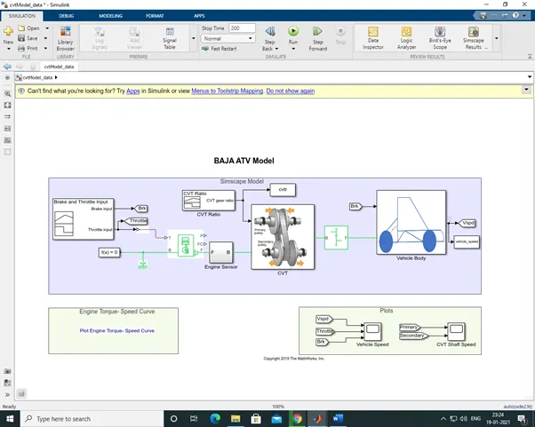
The final model of ATV using to workspace data will look like this-
*********************************************************************************************************************************************************************************************************************************************************************************************************************************************************************************************************************************************************************************
ATV Model with Dashboard
As we have seen in the previous model of CVT we had used the step block for providing the input signals for brake and throttle, in this model instead of set block & signal builder block we are giving the input signals of brake and throttle by using constant block & we will link this constant blocks with the knob , so that we can change the input of brake & throttle while the simulation is running.
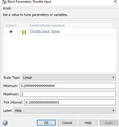
For this we will take 2 constant blocks and assign the constant blocks for brake & throttle . After this we will take 2 knobs from dashboard library, for linking the knob or connecting the knob with the constant block double click on the knob block a new window will open of bock parameter in that we can see the connect option in that , lick on connect after that click on any other Simulink block with which it is to be connected , here we have to connect the 2 knob blocks with the brake & throttle input constant block , so we will connect or link this constant blocks of brake & throttle with it respectively.
We will set the parameter of throttle knob as below shown in fig-
We will set the parameter of brake knob as below shown in fig-
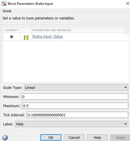
After connecting this throttle knob & brake knob with throttle & brake input respectively we use custom Gauge block for displaying the engine rpm and vehicle speed or velocity.
For this we will take 2 custom gauge and link them with the engine rpm and final velocity output blocks from the model.
The dashboard will then look like as shown in below fig-
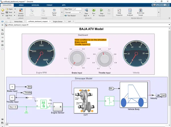
After this the outputs are taken from both the constant block respectively and the break output is given to GOTO port so that it can be used to connect easily to any other port easily without showing connection lines & the output of throttle is given to the generic engine T port by using Simulink to PS converter as the signal builder is and Simulink model and generic engine is and physical block or simscale block , so we cannot connect it directly so this Simulink to PS converter block is used, Also the throttle output is given to GOTO port for easy connection with other system.
The generic engine is an simple block representing an engine it consists of five ports, port T is input port for throttle input to which the signal of throttle of signal builder is given and Connections F and B are mechanical rotational conserving ports associated with the engine crankshaft and engine block, respectively. Connections P and FC are physical signal output ports through which engine power and fuel consumption rate are reported.
The F port which is an mechanical conversion port of speed of engine crankshaft is given to other subsystem called engine sensor to sense the speed /rpm of engine the B port is connected to the solver configuration and a mechanical reference is also connected to this B port as its and mechanical part , so this solver configuration and mechanical ports are important ports for running simulation successfully.
The input parameters for generic engine such as speed vector and torque vector are given by creating an variable in workspace as speedVector and torqueVector
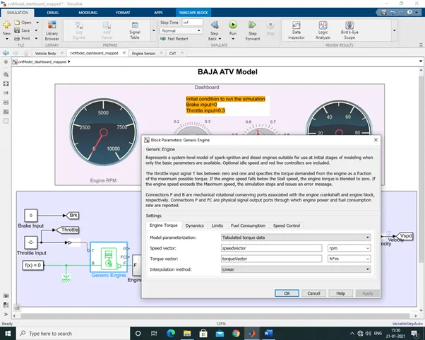
As shown in below fig the variables are created in workspace and the input values are assigned for speed vector and torque vector respectively.
This is the graph which is showing the engine speed torque curve :-
We can se in above graph that the engine speed is starting from 1500 rpm and going upto 3800 rpm and torque is from 6Nm to 22Nm.
This is how the blocks are connected as per this condition-
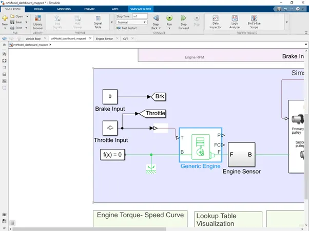
The output of generic engine block F port is connected to ideal rotational motion sensor to R port of it to sense the rpm of crankshaft the ideal rotational motion sensor is nothing but only a sensor to sense the angular velocity, its consists of 5 ports the R port is the input port , Connections R and C are mechanical rotational conserving ports and connections W and A are physical signal output ports for velocity and angular displacement, respectively. The mechanical reference is connected to the C port of ideal rotational motion sensor and W port is connected to the scope to observe the rpm of crankshaft by using the PS-Simulink converter as the ideal rotational motion sensor is an ps block while the scope is an Simulink block , for connecting the W port with scope successfully this block is used. While A port of rotational motion sensor is connected to the PS terminator the use of PS terminator is to terminate physical signal outputs. Unconnected physical signal output ports do not generate warnings, but connection to a PS Terminator can be used to indicate that the signal was not inadvertently left unconnected. After creating this sensor model it’s the created to an subsystem for creating the simplicity in the Simulink model, there are two PMC port in this which enable Physical Modeling Connection Port block for subsystems PMC port 1 & 2 are the connection port for the subsystem.
The subsystem is named as engine sensor and if the subsystem is opened it looks like below as shown in fig-
The subsystem for engine sensor is been modelled now after sensing the engine rpm thr F port of the generic engine block is given to the variable ratio transmission block B port , , the variable ratio transmission Represents a variable ratio gearbox such as implemented by mechanical belt CVT, electric, or hydraulic transmissions. The physical signal input r defines the ratio of input to output angular shaft velocities.
Connections B (base) and F (follower) are mechanical rotational conserving ports.
The output of generic engine F port is connected to B port of variable ratio transmission through engine sensor subsystem output port B , to the input B port of variable ratio transmission a ideal rotational motion sensor and inertia block are connected to sense the angular motion and to provide a inertia to the base of variable ratio transmission , the R port of ideal rotational motion sensor is connected to the base of variable ratio transmission B port and C, W & A port of ideal rotational motion sensor are connected to the mechanical reference block, scope with the help of PS-simulink converter block and PS terminator block respectively.
The other port of variable ratio transmission block i.e- F port (follower) is taken out , to this also a ideal rotational motion sensor is connected to sense the angular motion of sensor , this is connected in similar manner as the previous rotational sensor was connected to the base of variable ratio transmission, also for this port the inertia block is connected to provide inertia . the inertia block doesn’t have any operation related to this system only the help in configuring the system.
Here the 2 variables are created that are m1 & m2 for the values of inertia of base and follower of variable ratio transmission block respectively. The values of m1 & m2 are set as 3.5 and 3.2 respectively.
The angular motion that we have sensed for the base and follower are named as primary and secondary rpm respectively. The output of this both the rotational sensors are connected to the GOTO port (W was the output port of this sensors)
The subsystem of CVT will like this-
In previous model of CVT we used a signal builder block which gave the input signal to the R port of variable ratio transmission block here instead of signal builder block we are using a look up table block ,
The PS Lookup Table block computes an approximation to some function f=f(x) given data vectors x and f. Both the input and the output are physical signals.
The length of the x and f data vectors provided to this block must match. Also, the x data vector must be strictly monotonic, either increasing or decreasing.
Plotting a lookup table lets you visualize the data before simulating the model, to make sure that the table is correct. The plot reflects tabulated data specified for the block, as well as the selected interpolation and extrapolation options.
For setting the look up table there is need to provide the values for table grid values and table values the values are entered in this block by creating the variables for it the variable which is created for values of table grid is named as vehicle speed and this values which are specified for vehicle speed in the workspace is further divided by 3.6
And the variable which is created for table value is named as cvtr.
The variable which are created for vehicle speed and cvtr in workspace window are like this-
The look up table will look like follow-
Now the model is been modelled upto the simple gear block which in real life model is differential ,further we have to give this signal to the final drive that is wheels of the vehicle body , for that we have to model further the model of vehicle body
The model of Simulink will look like follow till now-
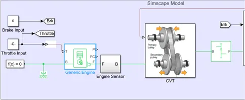
Now we have to modal a vehicle body or vehicle body subsystem:-
For this we will be using –
- Vehicle body block
- Tire block (4 blocks of tire)
- Double shoe brake
This 3 are some important blocks for modelling a vehicle body subsystem.
The subsystem of vehicle body looks like below-
The vehicle body as 6 ports ,
connection H is the mechanical translational conserving port associated with the horizontal motion of the vehicle body. The resulting traction motion developed by tires should be connected to this port.
Connections V, NF, and NR are physical signal output ports for vehicle velocity and front and rear normal wheel forces, respectively.
Connections W and beta are physical signal input ports corresponding to headwind speed and road inclination angle, respectively.
The vehicle body look like this-
The parameter for vehicle body are set as follows-
The NR port of vehicle body is the rear axle port and we have set the number of wheels per axle as 2 so we will connect 2 tires to this NR port , this NR port will be connected to the N port of tire as N port is the physical signal input port. In similar manner the NF port is connected to the 2 tire blocks in similar manner.
The tire block as 4 number of ports as A, N, H & S
Connection A is the mechanical rotational conserving port for the wheel axle.
Connection H is the mechanical translational conserving port for the wheel hub through which the thrust developed by the tire is applied to the vehicle.
Connection N is a physical signal input port that applies the normal force acting on the tire. The force is considered positive if it acts downwards.
Connection S is a physical signal output port that reports the tire slip.
The tire block looks like follow-
To both the rear tires the output of simple gear follower is connected to the A port of both the rear tire i.e left rear and right rear . there will be no direct drive from follower of simple gear to the front axle or wheels. Also the inertia and double shoe brake are connected in between the F port simple gear and A port of tire block.
The double shoe brake has 2 ports-
Connection S is a conserving rotational terminal associated with the drum shaft.
Connection F is a physical signal port representing the force input to the actuator. Positive force creates friction torque that resists shaft rotation.
The input of brake are taken from step block and given to input of the brake shoe F port with the help of from block and then sent inside the subsystem of vehicle body with the help of inport block. Then this signal from inport block are given to the gain block which will multiply the input force , to connect this gain block with the F port of double shoe brake a Simulink to PS converter block is used.
The connection will look like this-
The A ports of front tire i.e left front and right front will be connected to the rotational free end block.
The connection of A port of front wheels will like this-
The input parameters for all the 4 tires are set as default , no any changes are made in parameters of tire.
The H port of left rear and left front are connected with each other as H port is the mechanical translational conserving port
While the H port of right rear and front front are connected with each other as H port is the mechanical translational conserving port, and S port of all 4 tires are connected to PS terminator individually.
A PS constant blocks are used to connecte the W & beta ports of vehicle body. The PS constant block are set as 0 for both W & beta input values.
The V port of vehicle body block is the output port for vehicle velocity as we have discussed earlier so this block connection is taken out of subsystem with the help of output port and along with this the signal of velocity is given to the look up table input F port , as we have discussed earlier while describing the look up table , so that now the close loop is been formed between the model. The signal of V port of vehicle body which we have taken out of the subsystem is connected to GOTO port so that it can be connected to the scope for viewing results without showing the connection lines. This GOTO port is named or tag as Vsped.
Now all the GOTO ports of throttle , brake , Vehicle speed , cvtr, primary and secondary are connected to the scope with the help of from block to the scope,
There are three scops at the end for viewing results , for first scope the outputs or results of vehicle speed , throttle and brake are displayed and in the second scope the graph of primary and secondary rpm of CVT are is been observed. And in the third scope the result/graph of cvt is observed.
The first scope is been named as Vehicle speed and the second scope is named as CVT shaft speed and the third scope is named as CVT ratio .
Note – before running the simulation we have to set the simulation time or stop time to infinity(inf)
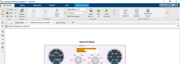
After clicking the run button we are able to change the brake & throttle input by turning the knob switches .
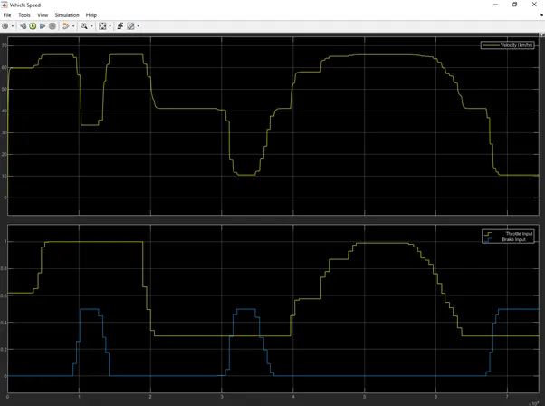
The result of vehicle speed scope are as shown in below fig-
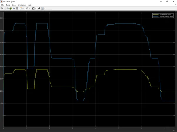
The result of CVT shaft speed scope are as shown in below fig-
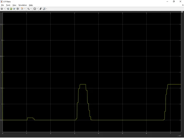
The result of CVT ratio scope are as shown in below fig-
Conclusion :-
By using the knob and custom gauge blocks and linking it with the brake , throttle , engine rpm & velocity blocks we are able to simulate the ATV model similar to a real life conditions.