Project

BAJA ATV CVT MODEL

AIM :

Our aim is to carry out the system level simulation of the Baja ATV (All Terrain Vehicle) and prepare the technical report explaining the different types of models and their properties. Also, observe the plots at different situations and comment on the results.

OBJECTIVE :

Model 1

Carry out the simulation of the Baja ATV with the CVT (Continuous Variable Transmission) model using signal builder for gear ratio.

Model 2

Carry out the simulation of the Baja ATV with the CVT gear ratio selected using a lookup table.

Model 3

Carry out the simulation of the Baja ATV with CVT model using the dashboard.

Model 4

Carry out the simulation of the Baja ATV with CVT model using the dashboard and the lookup table visualisation by mapping the CVT ratio with respect to velocity of the vehicle.

THEORY :

Continuous Variable Transmission(CVT):

CVT allows the engine to operate at optimum power and efficiency at varying conditions. At different conditions of speed, RPM and load, the CVT changes the gear ratio and allows the engine to work constantly.

The basic components of CVT are:

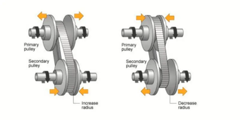
1. Drive pulley connected to engine (Primary pulley).
2. Driven pulley connected to axle (Secondary pulley).
3. Variator.
4. Belt.

In this the variator changes the radius of the primary and secondary pulley according to the required conditions and thus it changes the speed of the vehicle.

So, as we increase(press) the throttle, the variator narrows the primary pulley, which means there is increase in the radius of the drive pulley and widens the secondary pulley. This creates a higher gear ratio and allows it to reach higher speeds.

In the same way, as we release the throttle. The radius of the primary pulley is less than the radius of the secondary pulley, which reduces the gear ratio and in turn reduces the speed of the vehicle.

CVT

MODEL 1 :

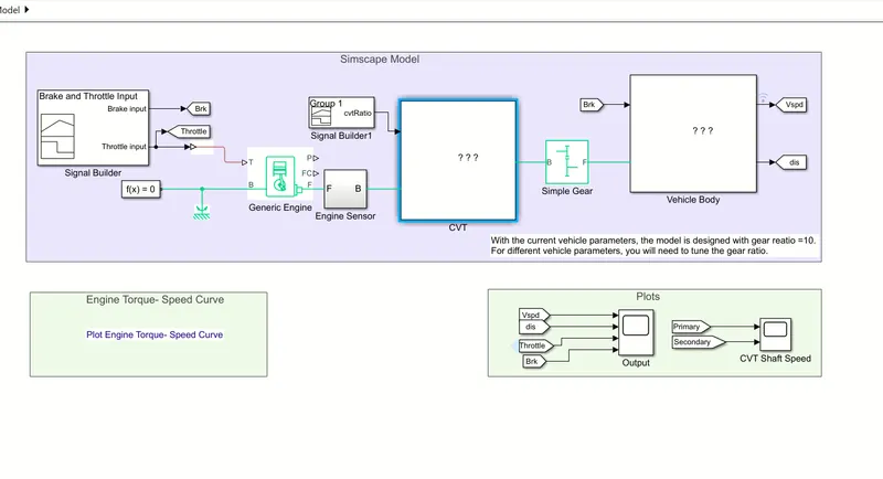
Simscape model

Signal Builder

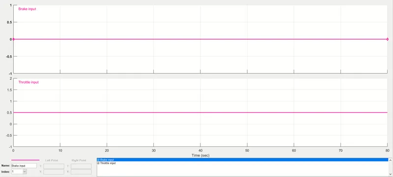
The signal builder allows us to create a group of signal sources and insert them into the model. Also we can define the output waveform by the input signal. In this we created signal sources of Throttle and Brake.

Throttle and Brake input

Throttle :

It can be defined as a device used to control the flow of fuel or power to the engine. When the throttle is pressed, the power is supplied to the engine and by that the speed is increased. Here, we have given the throttle or also known as acceleration of 0.5 as input to the Baja ATV.

Brake :

It is nothing but the device used to totally halt the vehicle or to cut the power supply to the engine. So, as we are studying the torque and speed characteristics of the vehicle, the brake input here is 0.

Generic Engine :

Here it represents a system level model of diesel engine with the basic parameters.

The input signal T is a throttle which has the value lies between zero and one. It provides the necessary torque and speed to the vehicle.

Connections F and B are mechanical rotational conserving ports associated with engine shaft and block respectively.

Connections P and FC are physical signal output ports through which engine power and fuel consumption rate is calculated.

So, here the input signal (throttle) which is created in the signal builder is given as input to the generic engine. As we are focussing on the speed as the main parameter, the RPM sensor is taken in the generic engine from the port F and this is given input to the CVT variable gear ratio. So, according to the throttle input and with the help of a speed sensor, the CVT variable gear ratio can be detected and accordingly given to the vehicle.

Variable Ratio Gear:

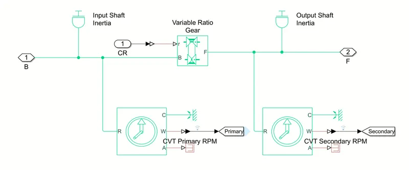
CVT SUBSYSTEM

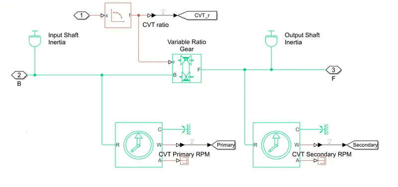
It represents a variable ratio gearbox implemented by mechanical belt CVT, electric transmissions. The physical signal input r defines the ratio of input shaft and output shaft angular velocities.

Connections B and F are mechanical rotational conserving ports. Here, we can consider them as the CVT primary RPM and the CVT secondary RPM. Therefore the difference between the primary RPM and the secondary RPM is mainly dependent on the variable ratio gear.

As this model is an open loop model, here the variable ratio input is given by the user with the help of signal builder block.

Simple Gear:

It represents a gear box. Here, with the vehicle parameters the gear ratio is taken as 10. Connections B and F are the mechanical rotational conserving ports. The vehicle body and the CVT block are connected by using the simple gear. So, as the gear ratio increases, the speed of the vehicle increases.

As the weight of the vehicle acts as an important parameter for the speed variation, the different vehicle parameters have different gear ratios. By observing the speed torque signal characteristics of the engine, one can select the gear ratio by trial and error method also.

Vehicle body:

It represents a two-axle vehicle body in longitudinal motion. This block accounts for the body mass, aerodynamic drag, inclination and the tire friction.

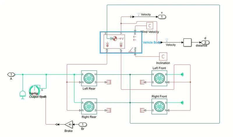
VEHICLE BODY

Connection H acts as the mechanical translational conserving port. As the name translation suggests, it is associated with the horizontal motion of the vehicle. All the tires traction motion is connected to this port as shown in figure.

Connections V, NR and NF are the physical signal output ports. V represents the vehicle velocity and by integrating this velocity signal we also get the distance.

Whereas NR and NF are the normal wheel forces on the front and rear end of the vehicle tires.

Connections W and beta are the physical signal input ports which are associated with the wind speed and the road inclination angle respectively.

Tire (magic formula):

It represents the physical vehicle tire, which is characterised by the tire magic formula. Here each axle has the two tires in the rear end and the front end of the vehicle body.

Connection A is the mechanical rotational conserving port for the wheel axle. As it represents the rotational motion, the output shaft and the gear ratio are connected to this port. Also a double shoe brake is used in this model.

Connection H is the mechanical translational conserving port through which thrust developed by the tire is applied to the vehicle. This makes the vehicle move in horizontal motion.

Connection N is the physical signal input port that applies the normal force acting on the vehicle.

Connection S is the physical signal output port that reports the tire slip. Here, in this model all the tire slips are terminated.

RESULTS:

Torque - speed curve:

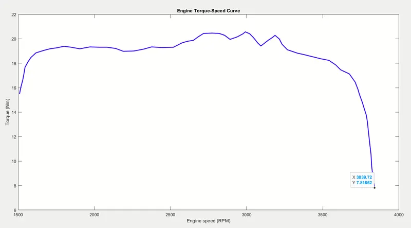
From the above figure we can see that the maximum speed attained by this vehicle is 3840 RPM. So, based on these parameters, the gear ratio of the model is taken as 10.

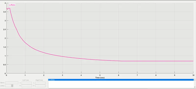
CVT Gear Ratio:

Primary & secondary RPM:

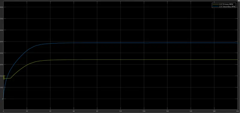
From the above curves, we can observe that, as the CVT ratio is getting below one, the secondary RPM of the shaft increases more than the primary RPM. And at constant ratio, the shaft attains the maximum RPM and flows constantly.

OUTPUT:

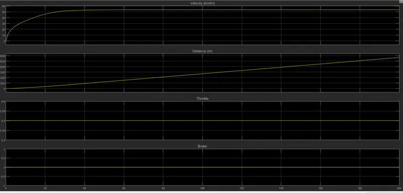
As the throttle input of 0.5 is applied, the velocity of the vehicle is increasing and attains the maximum velocity at 25 seconds. Here the brake input is given zero. And if we applied the brake at any time, the velocity curve would decrease to zero.

Model 2:

Simulink model:

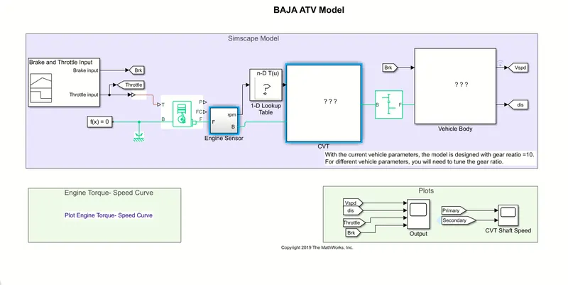
The only difference between the model 1 and model 2 is that model 2 has the 1-D lookup table whereas model 1 has the signal builder for CVT ratio.

THEORY :

Lookup table :

The table is a sampled representation of a function in N variables. The table data and the breakpoints relate the input values to positions. For example, here in our model the CVT ratio values and the speed variables are given as the input values.

This data can be extracted from the respected graphs or curves and can be stored in the workspace as excel sheet data.

Here. The CVT ratio values or data is obtained from the curve in the model 1. Also, we have the RPM sensor in the engine block from which we have collected the data for the speed variables that are given as input to the lookup table.

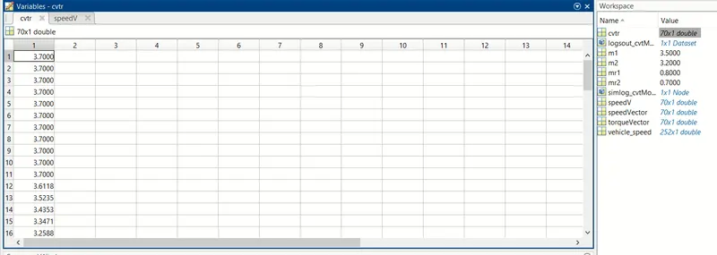
CVTr variables

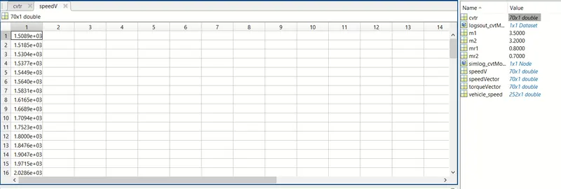
Speedv Variables

Engine sensor RPM :

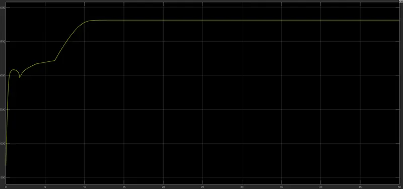
By using this curve, the speedv variables are obtained. As we can see from the curve, the starting RPM is about 1508 and the maximum RPM it has obtained is 3840.

GRABIT :

By using this Grabit file extension, we can extract the data points from the graph or curve. We can extract data points from any image file. After extracting the required points or variables, then these variables are fed into the system using the model workspace.

Also, the output results are the same as from model 1 as the only difference from model 1 is the lookup table and the data variables.

MODEL 3

Simulink model :

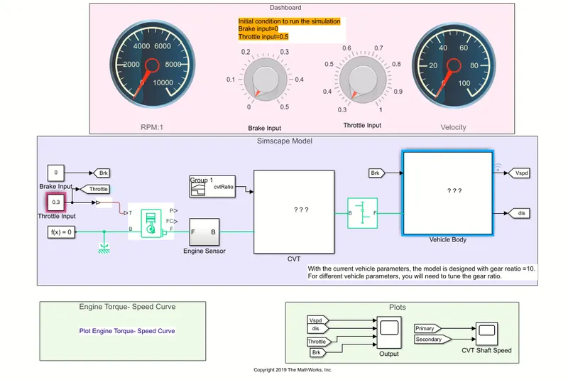
Dashboard :

In this model, we use the dashboard for the vehicle control. The user can control the input from the dashboard during the run time of the model. Here we have selected the stop time as infinity (inf) so that the user can apply the required throttle or brake input as when required to study the vehicle parameters at different conditions in a real time world.

In this model, we used the circular gauges for the representation of velocity and RPM of the vehicle. We also used Knobs for the brake and throttle inputs.

Also the initial conditions are mentioned to run the simulation as

Brake input = 0

Throttle input = 0.5.

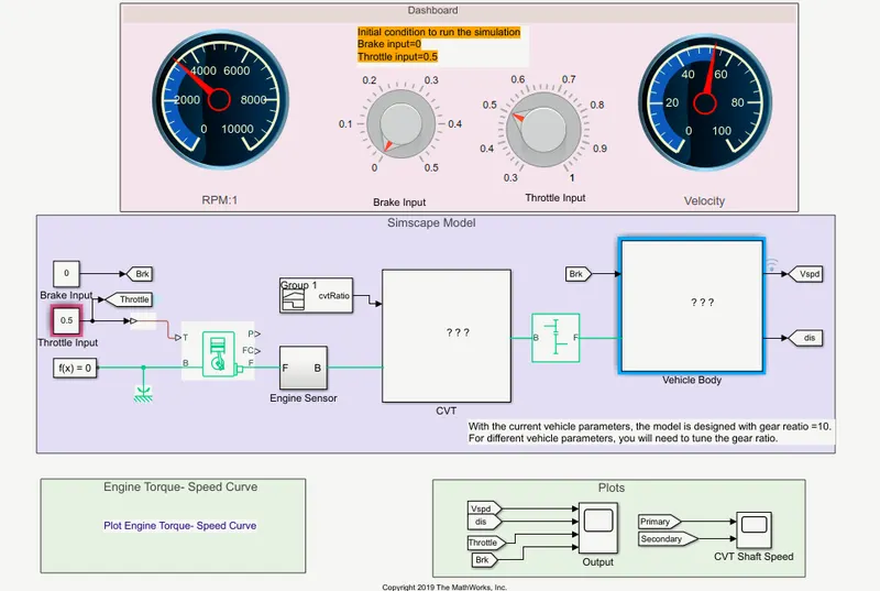
The above figure shows the dashboard during the simulation run time. As we can see the knob of the brake input is set at 0 and the knob of throttle input is set to 0.5.

We can also see the velocity gauge reaching the maximum velocity to almost 53 kmph and the maximum RPM shown is about 3840.

So, here also we have obtained the same output results by using the dashboard.

Model 4 :

Simulink model:

THEORY :

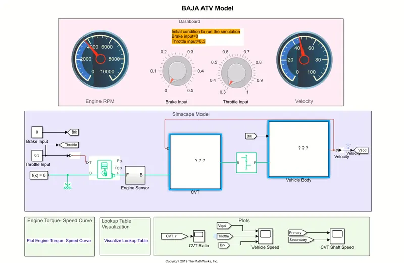
Above all the models are open loop type whereas this is the closed loop model. The velocity of the vehicle is again given as the input to the CVT block by using the lookup table. Here, we have mapped the CVT ratio with respect to change in velocity of the vehicle.

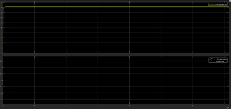
From the above figure in the dashboard we can see that the throttle knob input ranges from 0.3 to 1. So, based on the throttle input we get the data of the minimum and maximum velocity of the vehicle as Vmin = 41 kmph and Vmax = 65.9 kmph. So, according to this increase in velocity, the CVT ratio gets down and reaches the threshold value.

Lookup table map :

Lookup table visualise:

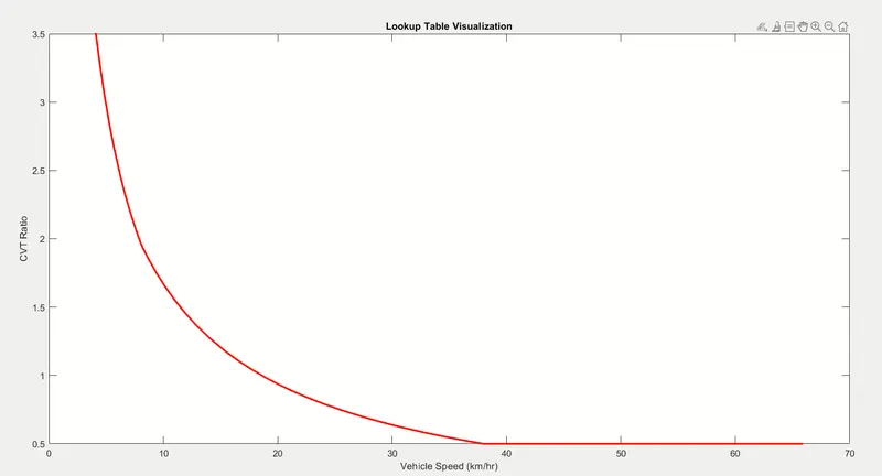
So, here the CVT ratio obtained is 0.5 at 37.97 kmph and remains constant as though there is change in velocity of the vehicle.

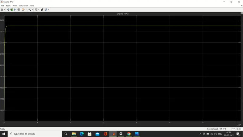
As, here we have taken the throttle input = 0.3 as the initial conditions, we can observe from the figure that there is decrease in vehicle speed to 41 kmph and the engine RPM to 2350.

RESULTS :

Engine RPM :

Throttle input and velocity: