Project
AIM
Carry out a system-level simulation of an all-terrain vehicle of the following models and analyse the results based on change in various input parameters
1)BAJA ATV model CVT gear without dashboard
2)BAJA ATV model CVT gear with dashboard of throttle and brake as input
3)BAJA ATV model based on CVT ratio from Engine RPM
4)BAJA ATV model - Data Extraction
5)BAJA ATV model with Mapped Lookup Table without Dashboard
6)BAJA ATV model with Mapped Lookup Table with Dashboard
THEORY
All Terrain Vehicle (ATV)
An all-terrain vehicle (ATV), also known as a light utility vehicle (LUV), a quad bike, or simply a quad,is a vehicle that travels on low-pressure tires, with a seat that is straddled by the operator, along with handlebars for steering control. As the name implies, it is designed to handle a wider variety of terrain than most other vehicles.
ATVs are intended for use by a single operator, although some companies have developed ATVs intended for use by the operator and one passenger. These ATVs are referred to as tandem ATVs.
The rider sits on and operates these vehicles like a motorcycle, but the extra wheels give more stability at slower speeds. Although most are equipped with three or four wheels, six-wheel models exists and existed historically for specialized applications. Multiple-user analogues with side-by-side seating are called utility terrain vehicle(UTVs)or side-by-sides to distinguish the classes of vehicle. Both classes tend to have similar powertrain parts.
Continous Variable Transmission(CVT)
The CVT is used to obtain infinite number of gear ratios in a certain range(For eg: 0.4 to 4). It consists of driver and driven pulleys of adjustable inner diameter so that gear ratios can be changed.The pulley is mounted over a shaft, which is input and output shaft.The input shaft connected from engine, the output shaft connected to transmission system.The steel belt is used as power transmission medium, so that when one pulley rotates it rotates another pulley.
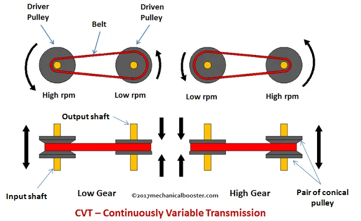
The above image shows the working of CVT. Initially assume the position of driver pulley having high rpm and driven pulley having low rpm. In this case, the diameter of driver pulley is adjusted to be less than driven pulley.This is the case in which output pulley rotates at lower speed than input pulley.This is a case of under drive.
To change the gear ratio, the input pulley and output pulley expand or collapse to adjust the suitable diameter so as to obtain desired gear ratio.
To obtain higher speed on output pulley, the input pulley diameter is adjusted to higher than output pulley.In this case, we achieve overdrive
BLOCKS USED
1)Signal builder: To create input for brake,throttle and cvt ratio. Braake and throttle input values changes from 0 to 1
2)GoTo block:To send signals to desired From block as per the requirement in program
3)From block: To obtain signals from GoTo block. From block can receive signals from multiple GoTo block. From block connect signals to scope block or to any other inport of a subsystem
4)Solve configuration: Defines solver settings to use for simulation
5)Mechanical Rotational Reference: This block represents a mechanical rotational reference point, that is, a frame or a ground. Use it to connect mechanical rotational ports that are rigidly affixed to the frame (ground)
6)Generic Engine: Represents a system-level model of spark-ignition and diesel engines suitable for use at initial stages of modeling when only the basic parameters are available. Optional idle speed and red line controllers are included.
If the engine speed falls below the Stall speed, the engine torque is blended to zero. If the engine speed exceeds the Maximum speed, the simulation stops and issues an error message.
Connections F and B are mechanical rotational conserving ports associated with the engine crankshaft and engine block, respectively. Connections P and FC are physical signal output ports through which engine power and fuel consumption rate are reported.
7)Ideal Rotational Motion Sensor: This block measures angular velocity or angle in a mechanical rotational network. The sensor is ideal since it does not account for inertia, friction, delays, energy consumption, and so on.
The physical signal ports W and A report the angular velocity and angle, respectively, of port R relative to port C. The measured angular velocity is positive when the angular velocity at port R is greater than the angular velocity at port C.
It is connected to engine crankshaft to measure engine RPM
8)CVT subsystem block: It contains 2 Ideal rotational motion sensor, 2 Rotational inertia,Variable Ratio Transmission block and inport block
8.a)Ideal rotational motion sensor:To measure input and output RPM of the shaft connected to input and output of variable gear ratio block
8.b)Rotational inertia: To indicate inertia value of shaft connecting input and output of variable gear ratio block. The mass m1 and m2 indicate masses of input and output shaft. The values of m1 and m2 are loaded from matlab workspace to calculate rotational inertia. Rotational inertia indicates input and output shaft
8.c)Variable Ratio Transmission: Represents a variable ratio gearbox such as implemented by mechanical belt CVT, electric, or hydraulic transmissions. The physical signal input r defines the ratio of input to output angular shaft velocities.
Connections B (base) and F (follower) are mechanical rotational conserving ports. Specify the relation between base and follower rotation directions with the Output shaft rotates parameter
8.d)Inport: To receive CVt ratio signal from signal builder and feed it to variable gear ratio block as input
9)Simple Gear: to connect CVt to Vehicle body, simple gear of specific gear ratio required. Gear ratio is set based on vehicle parameters
10)Vehicle body subsystem:It consists of
a)Inertia Output shaft: This shaft is from output of simple gear
b)Double shoe brake:It receives input at port F from inport 1 which receives brake signal from From block connected to subsystem.It represents a brake arranged as two pivoted rigid shoes symmetrically installed inside or outside a drum and operated by one actuator. The actuator force causes the shoes to exert a friction torque on a shaft connected to the drum
The other side S of brake is connected to 2 rear tyres
c)Tire (Magic Formula): Represents the longitudinal behavior of a highway tire characterized by the tire Magic Formula. The block is built from Tire-Road Interaction (Magic Formula) and Simscape Foundation Library Wheel and Axle blocks. Optionally, the effects of tire inertia, stiffness, and damping can be included.
The output port of 2 rear tyre are connected to double shoe brake,vehicle body,transmission system to front tyre and PS terminator.
The output port of 2 front tyres are connected to transmission system from rear tyre, vehicle body and PS terminator. One port of the 2 front tyre is rotational free end
d)Vehicle body:It receives input from front and rear tyres at NF and NR ports respectively.NF and NR are the wheel forces.The port H is connected to tyre transmission system.Connection H is the mechanical translational conserving port associated with the horizontal motion of the vehicle body. The resulting traction motion developed by tires should be connected to this H port.The port V from vehicle body gives velocity as output. On integrating the velocity v gives output as distance travelled by car during the simulation run time
1)WORKING OF BAJA ATV model CVT gear without dashboard
BLOCK DIAGRAM
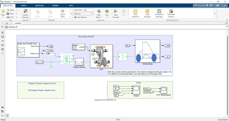
The brake and throttle input is provided as input.It is provided from signal builder block shown below
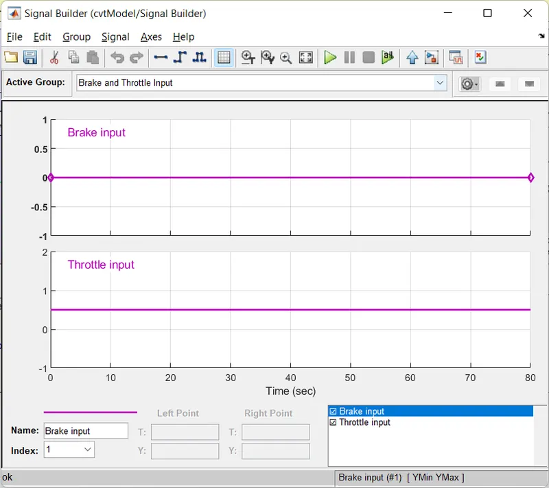
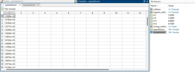
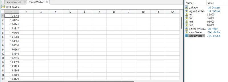
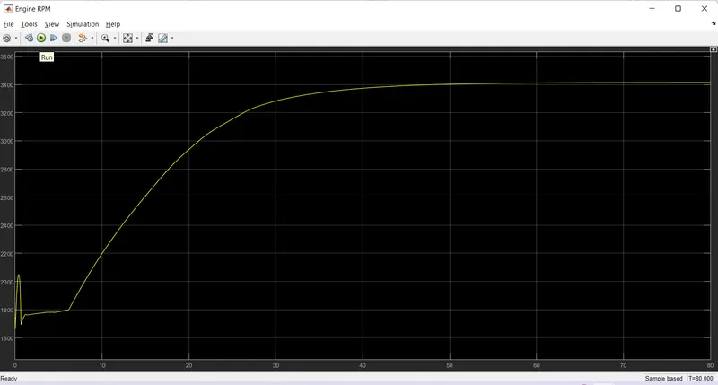
The generic engine receives throttle as input,throttle value=0.5.The brake input is received by double shoe brake in vehicle body subsystem.On receiving the throttle, fuel is burned in engine crankshaft and it generates output speed in RPM which is sensed by rotational motion sensor in engine sensor subsystem.This is the engine rotational speed. Here, the engine rotational speed,torque values are already calculated and plot in speed torque graph.The generic engine receives set of values of speed and torque as input, which is obtained from matlab workspace.Then it calculates the engine rotation speed against simulation time in engine sensor
The input 70 set of values of speed and torque are shown below
The engine speed during simulation time is shown below
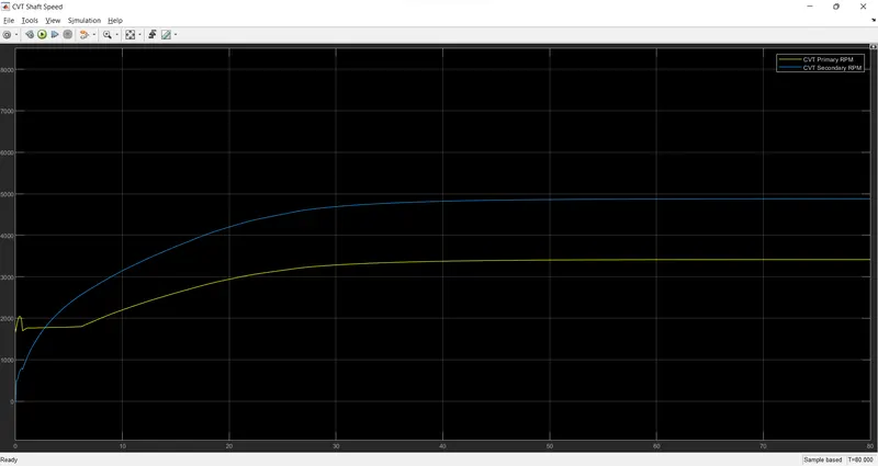
The engine sensor forwards the engine rotation to the shaft which is connected to input of variable gear. The input shaft is selected in such a way that engine RPM to be equal to rotational speed of the shaft.for that purpose, the suitable mass to be selected which is m1=3.5 kg.The rotational speed of the input shaft is measured using ideal rotation motion sensor which is marked as primary ain GoTo block. This shaft is the input shaft of variable gear. The rotational speed of output follower shaft is also measured which is marked as secondary in GoTo block. The primary and secondary RPM values are plotted against simulation time
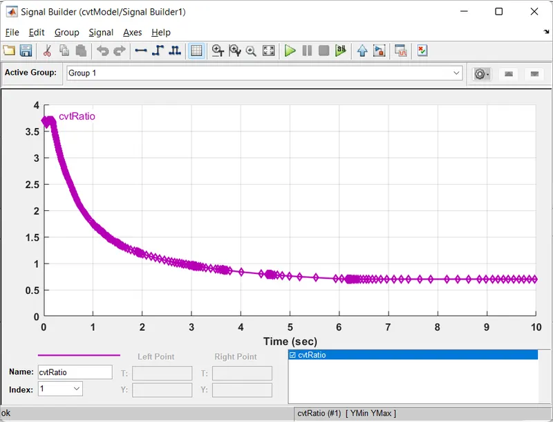
The variable gear ratio block receives various CVt ratio in 20 sec, which is shown below
The output follower shaft is connected to base of simple gear of gear ratio 10. The gear ratio is selected as 10 for the ATV vehicle of current parameter.The simple gear of certain gear ratio is required to connect CVt to vehicle body to have speed control. The vehicle body receives rotational output from the shaft of follower of simple gear as input to the 2 rear tyres. The vehicle body subsystem also receives brake input which is connected to double shoe brake. The double shoe brake then connects to the 2 rear wheel. The 2 rear tyres are connected to front tyres through transmission system at via H port. The wheel force and traction force between front and rear tyres are connected to vehicle body through NR,NF and H port. The velocity v output is obtained from vehicle body through V port. On integrating velocity over the simulation run time gives the distance travelled during that time interval
Significance of Engine torque-speed curve
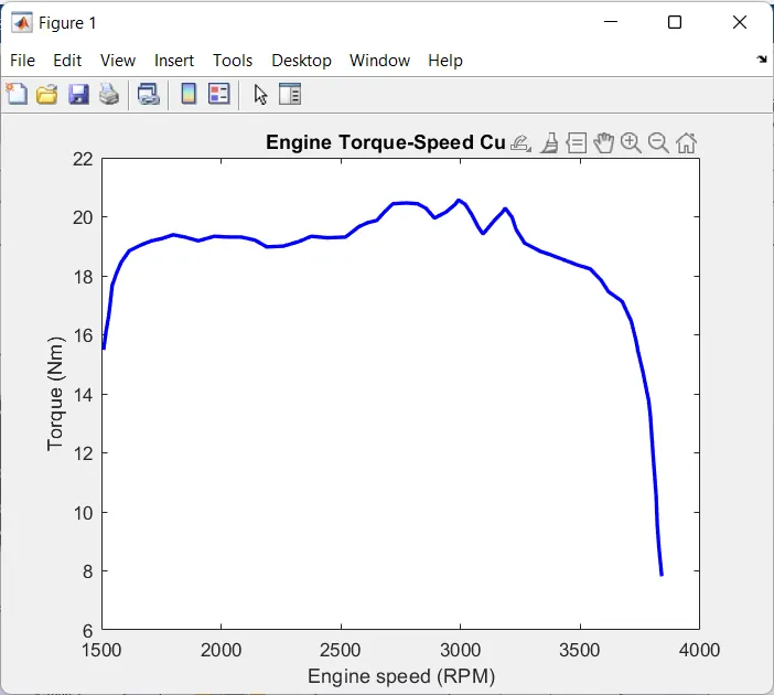
These are the physically obtained test values. The simulation result of engine RPM does not go beyond this range
RESULT
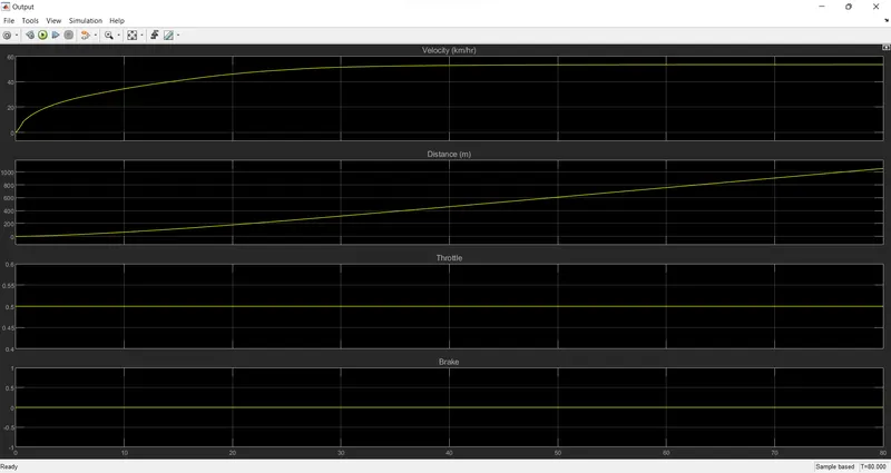
The below graph showing velocity and distance travelled for 80 seconds with throttle and brake as input. After 40 sec, the vehicle velocity remains constant
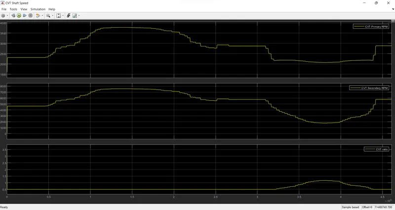
The graph below showing the variation of secondary shaft speed with respect to primary shaft during simulation time. These are the input and output shaft connected to variable gear. The output shaft having smooth variation of velocity
2)WORKING OF BAJA ATV model CVT gear with dashboard
Extra blocks used
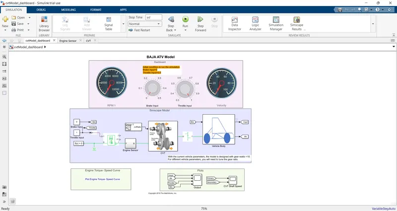
1) Knob: To provide varying brake and throttle input (In previous model, signal builder is used to give specific brake and throttle input). Here 2 knob were used
2) Circular gauge: To display engine rotational speed(RPM) and vehicle velocity.2 circular gauge were used
MODEL DIAGRAM
PROCEDURE
The knob of brake and throttle input are varied to see the simulation results. The simulation time is set to inf so that we get enough time to do the test and stop the simulation as per our convenience
RESULTS
The following graph below shows the variation of velocity based on change in throttle and brake values. as the vehicle is moving forward, the distance Vs time graph is continously increasing
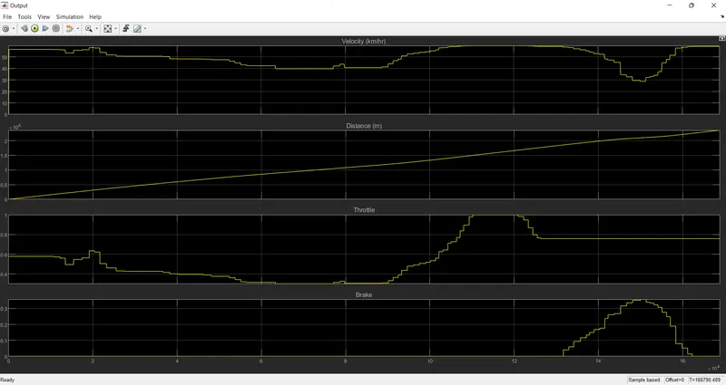
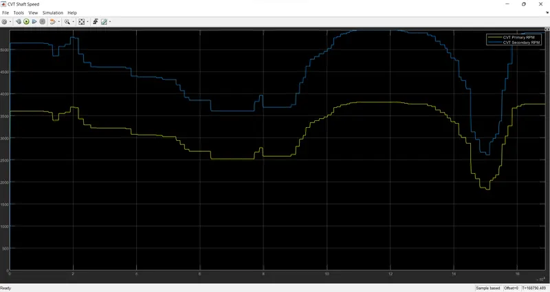
When the throttle is increased the vehicle velocity is increased and when throttle decreased the velocity decreases. When the brake value increased, velocity decreased and when brake decreased velocity increased. These are clear from the above graph. The situation is same for engine RPM also. As the engine is connected to primary input shaft of CVt, the same result. The primary shaft and secondary shaft speed variation graph is also similar to vehicle velocity graph.
The graph below shows variation of CVt primary and secondary RPM based on simulation time against change in brake and throttle values
3)WORKING OF BAJA ATV model based on CVT ratio from Engine RPM
The model diagram is shown below
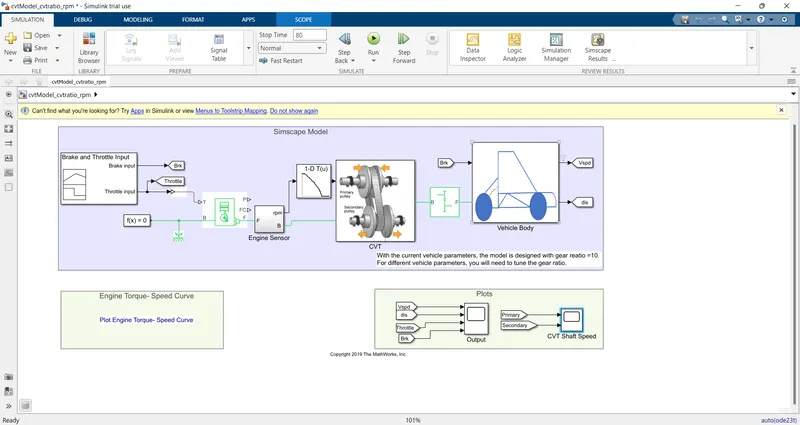
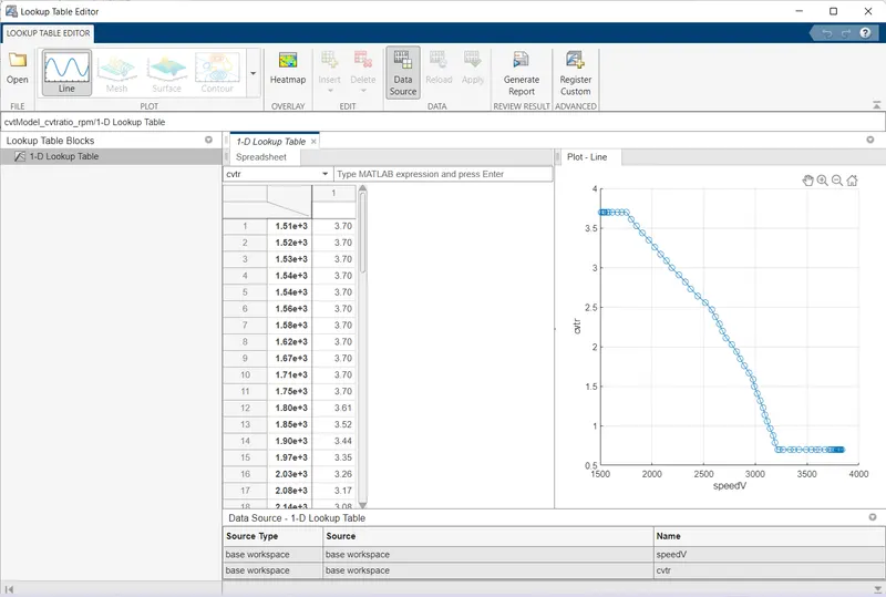
The difference from above 2 model is that it uses look-up table block. The look-up table receives engine RPM from engine sensor(Generic Engine). Based on engine RPM, the look-up table calculates the required CVt ratio and provide it as output to CVt subsystem. The CVt values were calculated from the set of values loaded from matlab workspace from the variable cvtr and speedV. The below diagram showing look-up table block. The matlab workspace variable and plot can be seen when we press Edit table and breakpoints in look up table block
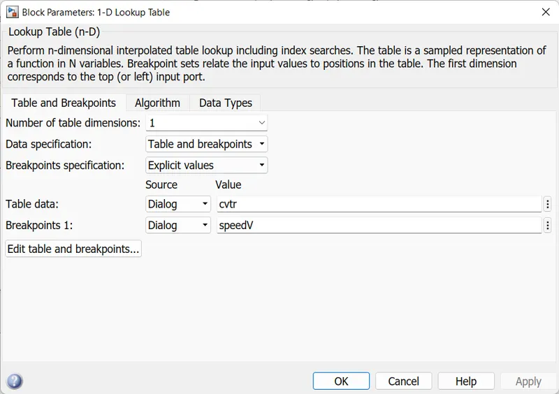
The CVtr vs Engine speed plot
RESULTS
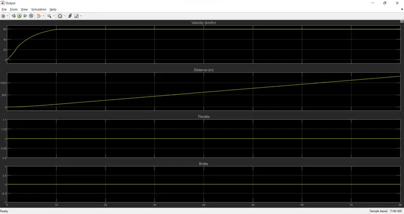
1)Velocity,distance,throttle,brake Vs simulation time
The graph is same as above model:1. The velocity remains constant after 10 sec because of throttle value 1
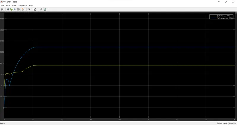
2)Primary and secondary shaft speed vs Time
The graph is same as above model
4)WORKING OF BAJA ATV model - Data Extraction
BLOCK DIAGRAM
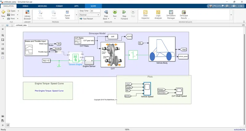
One modification in made in this block diagram is that CVTr ratio is also incorporated in scope block to study the variation of vehicle velocity as per change in CVT ratio
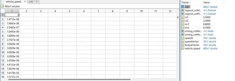
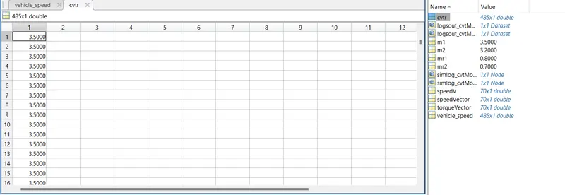
The main objective of this block is to extract CVT ratio and Vehicle speed to matlab workspace.CVT ratio and Vehicle speed data are extracted to matlab workspace using To Workspace block
INPUTS
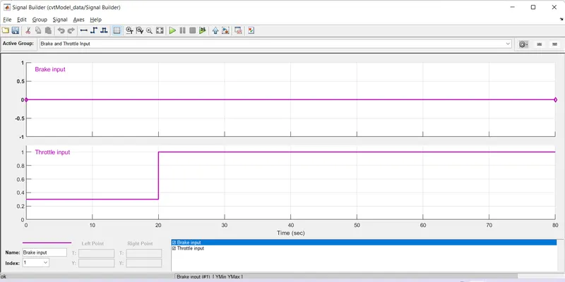
1)BRAKE and THROTTLE input
The throttle input value is 0.3 upto 20 sec. After 20 sec, throttle input changes to 1
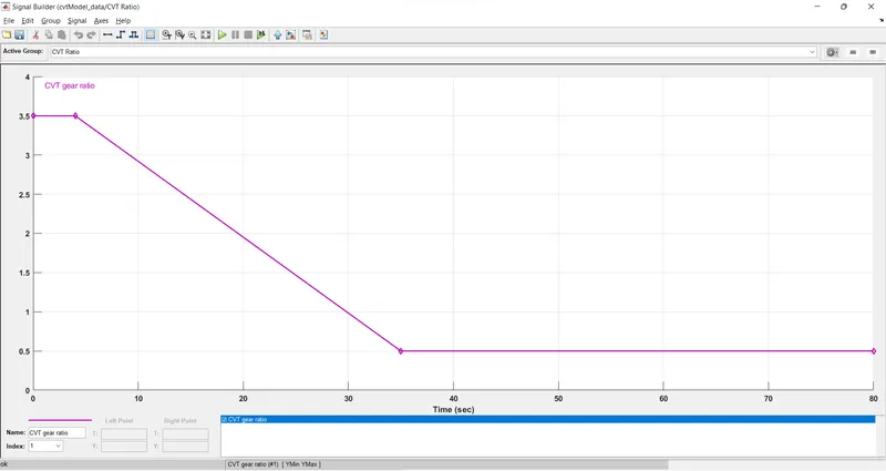
2)CVT ratio
OUTPUT
1) Velocity,throttle,brake and CVT ratio Vs Time (Simulation time 80 sec). The simple gear ratio used is 12 for this model
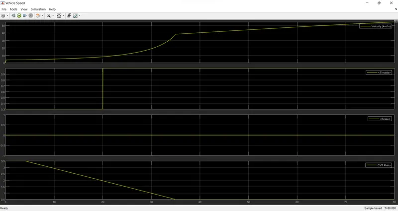
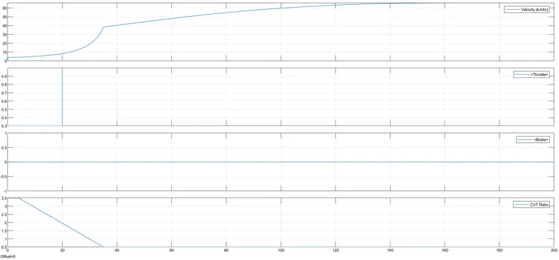
From 0-5 sec, the velocity is almost constant, because throttle value and CVT ratio are same.After 5 sec, the velocity values gradually increases, because CVTr values is gradually decreasing.At 20 sec, the throttle value suddenly changes to 1. So, from 20-30 sec, there is more increase in velocity values than compared to time range 5-20 sec.At 30 sec, the CVTr value approaches 1. So from 30-35 sec, there is sharp exponential increase in velocity values than from 20-30 sec. After 35 sec, there is a linear increase in velocity values upto 150 sec, then the velocity remains constant at around 65 kmph. This is shown in the figure below by changing the simulation time to 200 sec. The exact values of CVTr and Velocity values can be extracted from matlab workspace using To Workspace block as this is the main objective of this model
2)The primary and secondary shaft velocity Vs simulation time
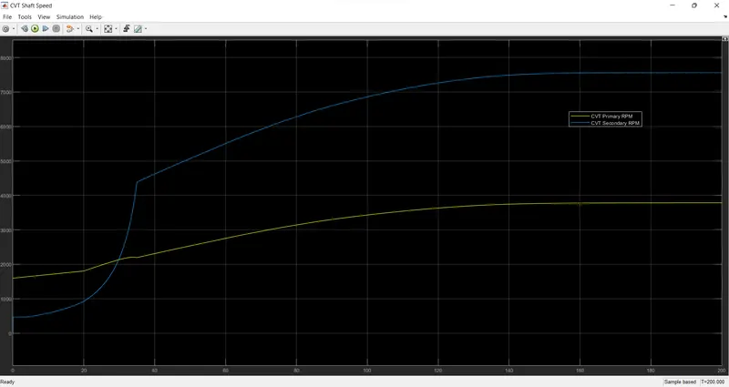
The secondary shaft RPM is similar to vehicle velocity
RESULT
1Vehicle speed variable extracted to matlab workspace
2)CVTr variable extracted to matlab workspace
5)WORKING OF BAJA ATV model with Mapped Lookup Table without Dashboard
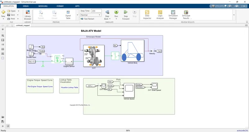
BLOCK DIAGRAM
PROCEDURE
Here the output velocity of the engine is taken and feed into CVT subsystem and then feed into look up table inside CVT subsystem. The figure below shows look up table connection block
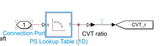
The look up table already have data sets of vehicle speed and CVT ratio. Based on input received as vehicle velocity, it calculates the CVT ratio required using interpolation or extrapolation methods. The interpolation and extrapolation methods, we can set in look up table. The PS look up table parameter shown below
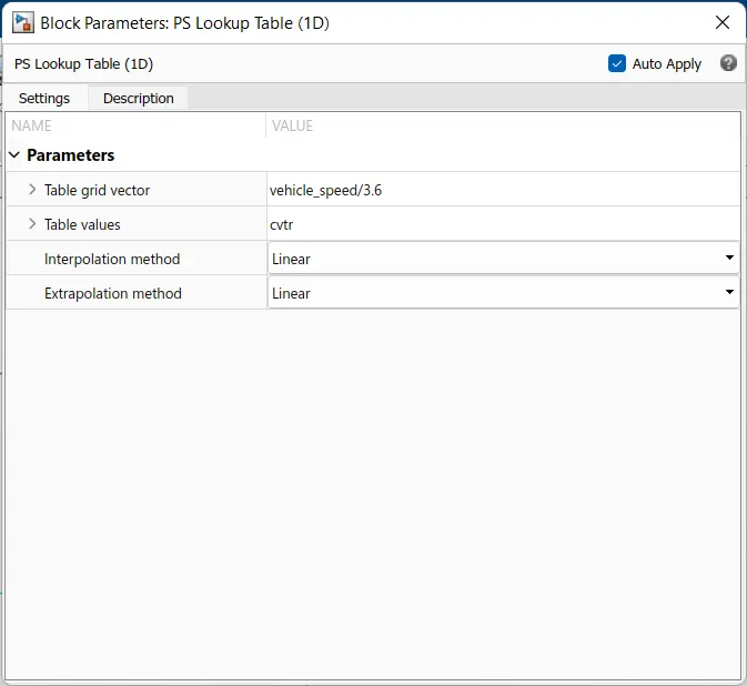
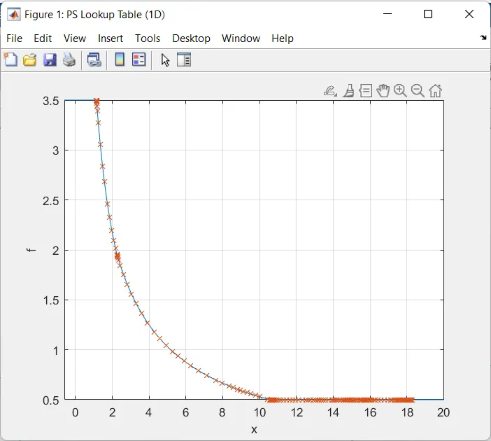
Vehicle speed and CVTr values are already defined in it. To see the values of vehicle speed and CVTr, right click on the look up table block and click on Foundation Library>Plot Table. The plot of Vehicle speed/3.6 vs CVTr values are shown below
The vehicle speed vs CVTr values can also be seen by clicking Vizualize Lookup Table in main block diagram
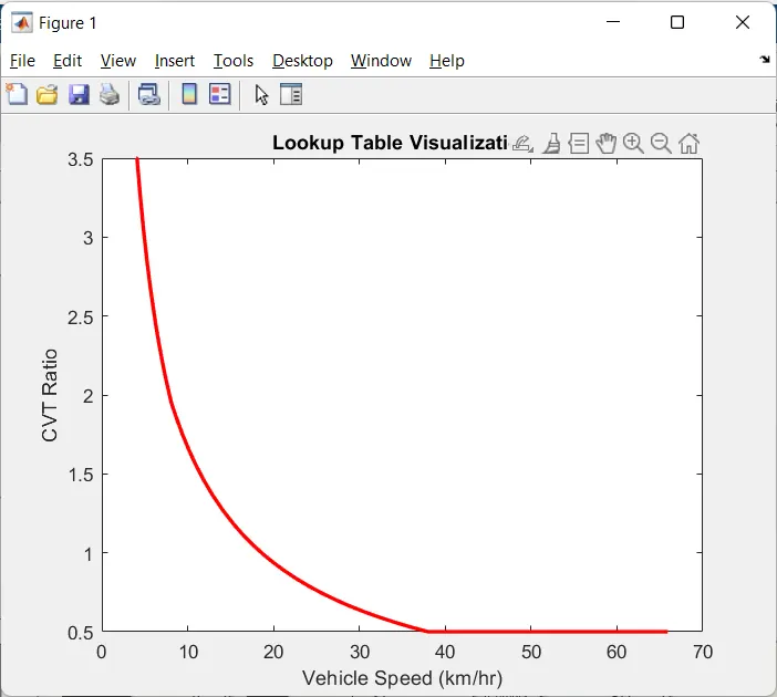
This data is feed into look up table as Table grid vector and Table values
RESULTS
The simple gear ratio is set to 12 for this model.
Vehicle speed,throttle input,brake input,CVT ratio vs Simulation time
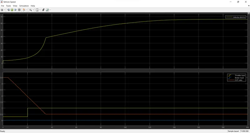
The result is similar to Model no:4 data extraction because the same throttle and brake input is applied. The look up table values are also similar to that of values extracted from Model:4.The only difference is that Vehicle velocity values start from around 4 kmph
6)WORKING OF BAJA ATV model with Mapped Lookup Table with Dashboard
BLOCK DIAGRAM
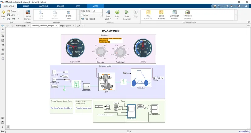
The simulation time is set to inf so that we get enough time to give varying brake and throttle input. All the other parameters are same as model:5
PROCEDURE:
The knob of throttle and brake is turned to get input values
RESULTS
The simple gear ratio is set to 12 for this model.
1)Vehicle speed variation wrt CVTr,throttle,btrake at simulation time inf
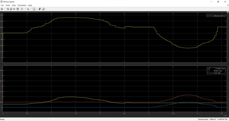
When the throttle input increases, the vehicle velocity increases and decreases in similar way.In this case, the CVTr value is constant 0.5.
When the brake input increases, the vehicle velocity decreases and reverses in the same way. The CVTr value is increased when the brake input value is increased, thus the velocity is decreased. The CVTr value is decreased when the brake input value in decreased, thus vehicle velocity increased.
Whatever happening to the vehicle velocity, the same thing happens to secondary shaft velocity of CVTr gear. This is shown in plot below