Project 1 - Parsing NASA thermodynamic data
1. Write a function that extracts the 14 co-efficients and calculates the enthalpy, entropy and specific heats for all the species in the data file. You will be reading this file NASA thermodynamic data(Tip: use fopen and fgetl). The formulae are shown below.
Here R is the universal gas constant, T is the temperature
The FIRST 7 coefficients are HIGH-temperature coefficients and the SECOND 7 coefficients are LOW-temperature coefficients.
Also use the LOCAL TEMPERATURE RANGES which is unique for each individual species, not the GLOBAL TEMPERATURE RANGE.
2. Calculate the molecular weight of each species and display it in the command window.
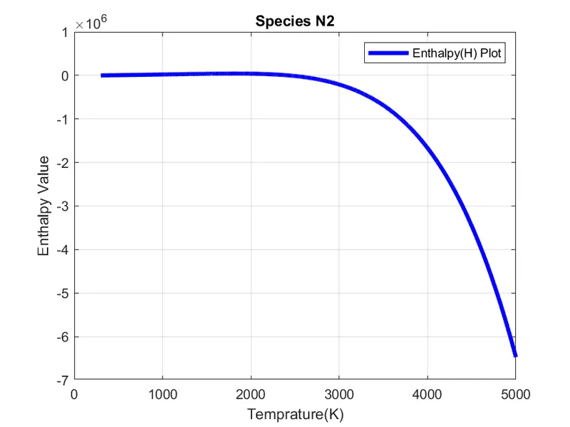
3. Plot the Cp, Enthalpy, and Entropy for the local temperature range (low temperature: high temperature) specific for each species.
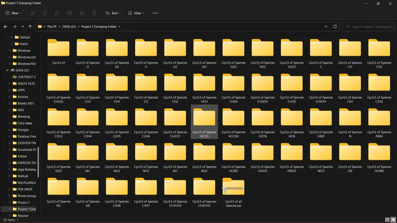
4. Save the plots as images with appropriate names and dump them in separate folders for each species with a suitable name. All these should be generated automatically.
5. The main program that you will submit will just take the "THERMO.dat" file as an input and generate Cp, H, and S plots.
6. Please write a detailed report to describe your logic.
Answers
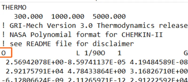
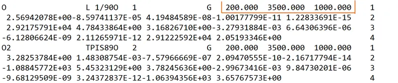
The data to be extracted from the NASA Thermodynamic data file are
- Species name
- Extracting local temperature ranges from the first line of each species
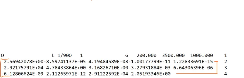
- Extracting coefficients from each species from lines 2,3,4 respectively.
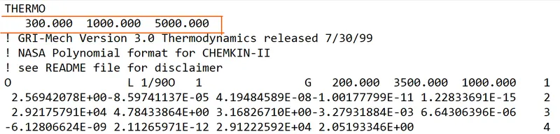
- Assigning global temperature range
Polynomial functions defined by NASA are defined below
`C_p=(a_1+a_2*T+a_3*T^2+a_4*T^3+a_5*T^4)*R`
`H=(a_1+(a_2*T)/2+(a_3*T^2)/3+(a_4*T^3)/4+(a_5*T^4)/5+a_6/T)*R*T`
`S=(a_1*lnT+a_2*T+(a_3*T^2)/2+(a_4*T^3)/3+(a_5*T^4)/4)*R`
Where,
T= Temperature in Kelvin
`(a_1,a_2,....,a_7)=`Coefficients given in the dat file
`C_p=`Coefficient of specific heat
H = Enthalpy
S = Entropy
The Matlab program to extract coefficients, plot Cp,H,S plots and save them in different folders is given below
clear all
close all
clc

% Step1
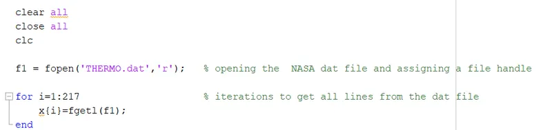
f1 = fopen('THERMO.dat','r');   % opening the  NASA dat file and assigning a file handle

for i=1:217                     % iterations to get all lines from the dat file
    x{i}=fgetl(f1);
end

% Step2
% Defining 53 species as a string to use it later
s ={'Species O' 'Species O2' 'Species H' 'Species H2' 'Species OH' 'Species H2O' 'Species HO2' 'Species H2O2' 'Species C' 'Species CH' 'Species CH2' 'Species CH2(S)' 'Species CH3' 'Species CH4' 'Species CO' 'Species CO2' 'Species HCO'  'Species CH2O' 'Species CH2OH' 'Species CH3O' 'Species CH3OH' 'Species C2H' 'Species C2H2' 'Species C2H3' 'Species C2H4' 'Species C2H5' 'Species C2H6' 'Species CH2CO' 'Species HCCO' 'Species HCCOH' 'Species H2CN' 'Species HCN' 'Species HNO' 'Species N' 'Species NNH' 'Species N2O' 'Species NH' 'Species NH2' 'Species NH3' 'Species NO' 'Species NO2' 'Species HCNO' 'Species HOCN' 'Species HNCO' 'Species NCO' 'Species CN' 'Species HCNN' 'Species N2' 'Species AR' 'Species C3H8' 'Species C3H7' 'Species CH3CHO' 'Species CH2CHO'};

% Step3
o=(6:4:217);    % Extracting species name for each species
p=(7:4:217);    % First row of coefficients for each species
q=(8:4:217);    % Second row of coefficients for each species
r=(9:4:217);    % Third row of coefficients for each species

% Step4
for m=1:53      % Iterations to extract all coefficients and Cp, H, S from the dat file

    n{m}=strsplit(x{o(m)});       % Reading the header line for each species
    t{m}=n{m}(1);                 % Creating species array

% Step5
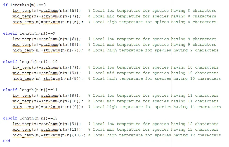
    if length(n{m})==8
        %s{j}=n{j}(1);
        low_temp{m}=str2num(n{m}{5});   % Local low temprature for species having 8 characters
        mid_temp{m}=str2num(n{m}{7});   % Local mic temprature for species having 8 characters
        high_temp{m}=str2num(n{m}{6});  % Local high temprature for spices having 8 characters

    elseif length(n{m})==9
        %s{j}=n{j}(1);
        low_temp{m}=str2num(n{m}{6});   % Local low temprature for species having 9 characters
        mid_temp{m}=str2num(n{m}{8});   % Local mid temprature for species having 9 characters
        high_temp{m}=str2num(n{m}{7});  % Local high temprature for species having 9 characters

    elseif length(n{m})==10
        %s{j}=n{j}(1);
        low_temp{m}=str2num(n{m}{7});   % Local low temprature for species having 10 characters
        mid_temp{m}=str2num(n{m}{9});   % Local mid temprature for species having 10 characters
        high_temp{m}=str2num(n{m}{8});  % Local high temprature for species having 10 characters

    elseif length(n{m})==11
        %s{j}=n{j}(1);
        low_temp{m}=str2num(n{m}{8});   % Local low temprature for species having 11 characters
        mid_temp{m}=str2num(n{m}{10});  % Local mid temprature for species having 11 characters
        high_temp{m}=str2num(n{m}{9});  % Local high temprature for species having 11 characters

    elseif length(n{m})==12
        %s{j}=n{j}(1);
        low_temp{m}=str2num(n{m}{9});   % Local low temprature for species having 12 characters
        mid_temp{m}=str2num(n{m}{11});  % Local mid temprature for species having 12 characters
        high_temp{m}=str2num(n{m}{10}); % Local high temprature for species having 12 characters
    end


% Step6
    for j=p(m):r(m)                 % Extracting coefficients from first and second row of each species
        y{j}=findstr(x{j},'E');     % Creating an array of strings to find 'E'

% Step7
        t1=1;                   % Defining starting point for each coefficient in the string

% Step8
        if j==r(m)              % For 3rd row there exist four 'E'
            for k=1:4           % Number of  iterations to extract vector from string
                t2=y{j}(k)+3;   % Defining ending of each coefficient in the string
                a1{j,k}=x{j}(t1:t2);        % Coefficients in string form
                b(j,k)=str2num(a1{j,k});    % Converting string to array
                t1=y{j}(k)+4;   % Increasing 't1' for next iteration
            end
% Step9
        else

            for k=1:5
                t2=y{j}(k)+3;   % Defining ending of each coefficient in the string
                a1{j,k}=x{j}(t1:t2);        % Coefficients in string form
                b(j,k)=str2num(a1{j,k});    % Converting string to array
                t1=y{j}(k)+4;   % Increasing 't1' for next iteration
            end

        end

    end


% Step10
% For Tlocal mid temprature

% Step12
    a_h(m,:)=[b(q(m),3:end) b(r(m),1:end-1)];        % Creating a row vector consisting coefficients specified for higher tempratures
    T_h=linspace(mid_temp{m},high_temp{m},3000);        % Higher temprature array for properties calculation
    RT_h=R*T_h;

% Step13
    Cp_h(m,:)=(a_h(m,1)+a_h(m,2).*T_h+a_h(m,3).*(T_h.^2)+a_h(m,4).*(T_h.^3)+a_h(m,5).*(T_h.^4))*R;       % Coefficient of Specific heat calculation

    H_h(m,:)=(a_h(m,1)+a_h(m,2).*T_h/2+a_h(m,3).*T_h.^2/3+a_h(m,4).*T_h.^3/4+a_h(m,5).*T_h.^4/5+a_h(m,6)./T_h).*RT_h;          % Enthalpy calculation

    S_h(m,:)=(a_h(m,1).*log(T_h)+a_h(m,2).*T_h+a_h(m,3).*(T_h.^2)/2+a_h(m,4).*(T_h.^3)/3+a_h(m,5).*(T_h.^4)/4+a_h(m,7))*R;     % Entropy calculation

    % Plots

% Step14
    mkdir(['D:\Project 1 Dumping Folder\Cp,H,S of ',s{m}])      % Creating  a folder directory to save the plot  figure

% Step15
    figure(1)       % Defining figure window
    plot(T_l,Cp_l(m,:),'linewidth',3,'color','r')        % Cp plot for lower temprature array
    hold on
    plot(T_h,Cp_h(m,:),'linewidth',3,'color','r')        % Cp plot for higher temprature array
    hold off
    legend('Specific heat(Cp) Plot')    % Defined legend to give plots a meaning full look
    title(s{1,m})     % Title of the window is specified as the cell array 's'
    xlabel('Temprature(K)')     % X-axis definition
    ylabel('Cp Value')          % Y-axis definition
    grid on

% Step16
    figure(2)
    plot(T_l,H_l(m,:),'linewidth',3,'color','b')         % Enthalpy plot for lower temprature array
    hold on
    plot(T_h,H_h(m,:),'linewidth',3,'color','b')         % Enthalpy plot for higher temprature array
    hold off
    legend('Enthalpy(H) Plot')      % Defined legend to give plots a meaning full look
    title(s{1,m})
    xlabel('Temprature(K)')         % X-axis definition
    ylabel('Enthalpy Value')        % Y-axis definition
    grid on

% Step17
    figure(3)
    plot(T_l,S_l(m,:),'linewidth',3,'color','g')     % Entropy plot for lower temprature array
    hold on
    plot(T_h,S_h(m,:),'linewidth',3,'color','g')     % Entropy plot for higher temprature array
    hold off
    legend('Entropy(S) Plot')       % Defined legend to give plots a meaning full look
    title(s{1,m})
    xlabel('Temprature(K)')         % X-axis definition
    ylabel('Entropy Value')         % Y-axis definition
    grid on

% Step18
    cd(['D:\Project 1 Dumping Folder\Cp,H,S of ',s{m}])     % Changing directory

% Step19
    saveas(figure(1),'Temprature VS Specific heat.png')      % Saving the plot in different folders
    saveas(figure(2),'Temprature VS Enthalpy.png')
    saveas(figure(3),'Temprature VS Entropy.png')
    pause(2)            % To get a glimpse of the plot
    close(figure(m))    % Close the figure window
end

% Step20
 for m=1:53      % Iterations to extract all coefficients and Cp, H, S from the dat file
    n{m}=strsplit(x{o(m)}); % To split the header string for each species
    t{m}=n{m}(1);           % Extracting species name
    l(m,:)=[t{1,m}];        % Making species array a row array
    Molecular_weight(l{m,1});   % Calling 'Molecular Weight'function to print molecular weight in command window
end- Step 1:
- Code starts with clear all, close all, clc to clean the previous garbage values.
- The motto of this program is to extract data from the 'NASA thermodynamic data' file to read and extract file, first of all the file needs to be in the same folder. fopen syntax is used to give the file a filehandle and use it to extract as required.
- The next step is to get each line as a form of strings so that everything is stored in a single array.
- The syntax fgetl is used to read each line from the NASA file, the for loop makes it a cell array where the cells are filled with each line which is present in data file. The strings get saved in 'x' array.
- Step 2:
- Created an array to make a species heading array where we use this in naming individual plots. Here the array consists of 53 cells of a row vector. As shown below

- Step 3:
- The next step is to create four-row vectors which repeat from each species. The first array 'o' array denotes the header for each species, 'p' array denotes the line2 of each species, 'q' array denotes the line3 of each species and 'r' array denotes the line4 of each species.
- The array has been made using the colon(:) operator.

- Step 4:
- The main part of this code starts with this for loop which runs for 53 iterations.
- The first step is to split each cell of 'x' array using syntax 'strsplit'
- Naming the first cell above is the species name. The species names can be extracted from the above cell.

- Step 5:
- As the length of molecules differs from each other some are larger and some are smaller ones, the length of each molecule define the starting position of local temperature and the temperatures follow a similar pattern. Species characters differ from 8 to 12.
- As first temperature term is local low temperature, the next one is the local mid-temperature, and the last one is the local high temperature.
- For different species as the starting position of local temperature differs we can use 'if-elseif' statements and define the position for every case.
- Three arrays have been created low_temp, mid_temp, and high_temp arrays where all the required local temperatures have been stored.
- The used syntax is str2num
- low_temp array=

- mid_temp array=

- high_temp array=

-
- Step 6:
- This step is to extract coefficients from each species. As the 2nd and 3rd lines are similar the same logic applies to both, so we run the for loop two times for each species.
- For this, we use findstr syntax to establish the position of E's in each line for each cell of x{j} and store the data in y{j} array.
- y{j} is a cell array that constitutes strings representing the position of E's in each line.


- Step 7:
- This step is to create a counter pattern of t1.

- Here, the counter pattern starts from a position of the first E and ends at the last one.
- Step 8:
- Each coefficient starts from the first position of a line(2,3,4) and end after three positions of respective E. The next coefficient starts from the fourth position after the first E and ends after the third position of the respective E. The repeating pattern is given below.
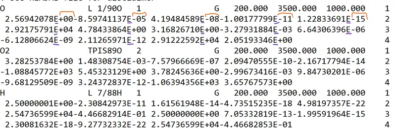
- The logic is to create a first term (t1) second term (t2) using position of E, then we create the characters where the coefficient is contained and we store this string in an array a1{j,k}.
- Then we convert the coefficients to vector using syntax str2num and store the vector in b-array.
- a1_array=
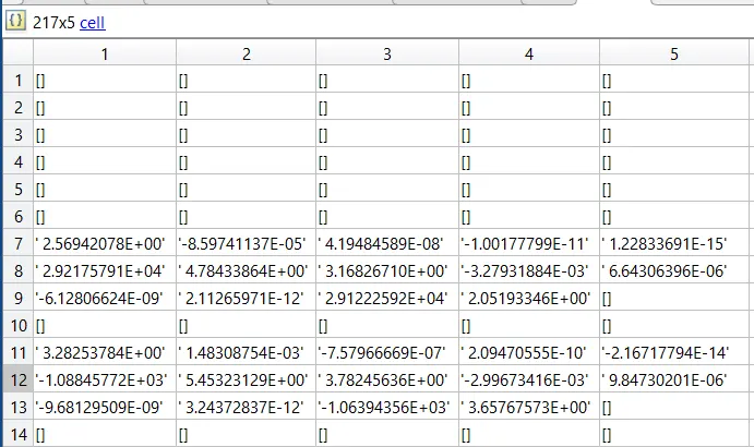 b_array=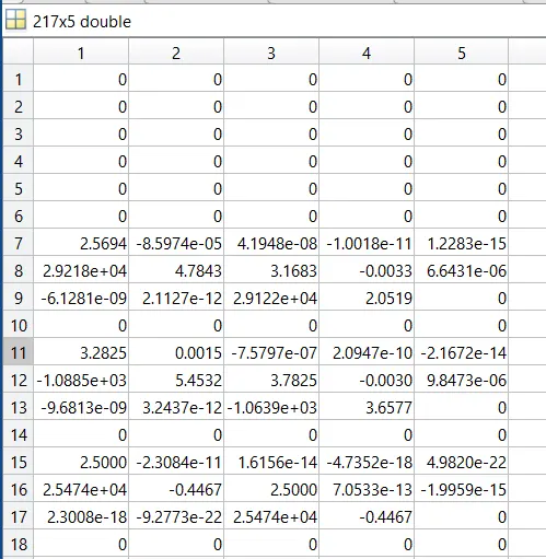
- From the above images, we can see that a1-array is a cell type array and b-array is a vector type array.
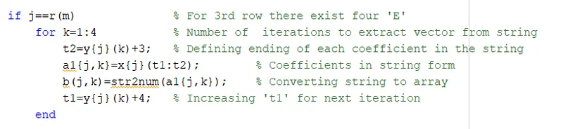
- The for-loop ends with a changed t1 value which ensures the position of E for the next iteration.
- The if-else statement here ensures the for-loop runs four times for the fourth-line of each species. Where there are only four coefficients as shown in the thirteenth and seventeenth row.
- Step 9:
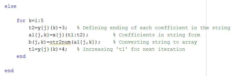
- The logic in this step is the same as above but the difference is this logic is for the 2nd and 3rd lines where there are five coefficients and five E's. This in turn boils down to a number of iterations which also becomes five.
- We get the result shown above in the image where we can see it clearly in a1_array and b_array.
-
- Step 10:
- The main motto here is to arrange the coefficients both for lower temperatures and higher temperatures, so we start with a_l-array.
- As the coefficients for lower temperatures are given in 2nd and 3rd lines, so to generalize we considered the p_array and q_array index the b_array in order to get a row vector with seven coefficients as each element.
- Assigned the value of the universal gas constant.
- The domain of the Cp, H, and S calculation has to be set. As this part is for lower temperature calculations we created a low-temperature array using the local temperature arrays. Using syntax linspace,2000 points have been created in between.
-

- Step 11:
- The equations for the Cp, H, and S have been calculated as given by NASA. Here we calculated for the lower temperature group.

- Step 12:
- This step is for higher temperatures and the same process as above is followed here as well.
- The domain of the Cp,H, and S calculation has to be set. As this part is for higher temperature calculations we created a high-temperature array using the local temperature arrays. Using syntax linspace,2000 points have been created in between.

- Step 13:
- The equations for the Cp, H, and S have been calculated as given by NASA. Here we calculated for the higher temperature group.
-

- Step 14:
- To create a new folder at desired location mkdir is used. Which creates new folders inside the destination folder. The syntax here creates unique folder names which will have the s{m} array elements at the end to make the folder less confused.

- Step 15:
- To plot the Cp VS T graphs the two different plot commands has to be executed
- 1st is Cp_l VS T_l, where Cp_l represents the specific heat coefficients for lower temperatures, which is less than the mid-temperature.
- 2nd is Cp_h VS T_h, where Cp_h represents the specific heat coefficients for higher temperatures, which is greater than the mid-temperature.
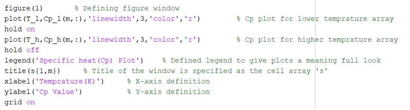
- To plot the Cp VS T graphs the two different plot commands has to be executed
- Step 16:
- To plot the H_l VS T graphs the two different plot commands has to be executed
- 1st is H_l VS T_l, where H_l represents the enthalpy values for lower temperatures, which is less than the mid-temperature.
- 2nd is H_h VS T_h, where H_h represents the enthalpy values for higher temperatures, which is greater than the mid-temperature.
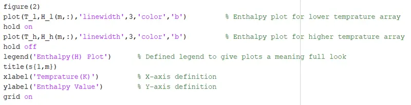
- To plot the H_l VS T graphs the two different plot commands has to be executed
- Step 17:
- To plot the S_l VS T graphs the two different plot commands has to be executed
- 1st is S_l VS T_l, where S_l represents the entropy values for lower temperatures, which is less than the mid-temperature.
- 2nd is S_h VS T_h, where S_h represents the entropy values for higher temperatures, which is greater than the mid-temperature
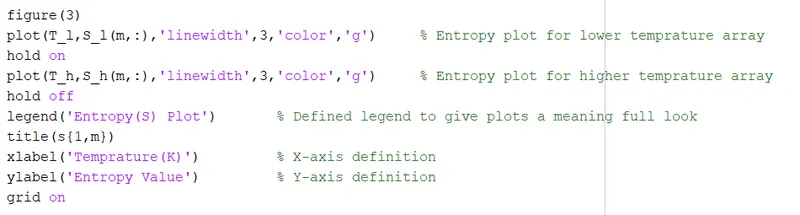
- To plot the S_l VS T graphs the two different plot commands has to be executed
- Step 18:
- The function cd is used to change the directory using a complete path and the following process occurs in the changed directory also the function is a global function if there isn't any folder then Matlab creates new ones and follows up processes occur.
- To change the folder name for each species we used the s{m}-array and made the folders more meaningful.

- Step 19:
- To save the plots for each species in one folder saveas function has been used. To save three plots we repeated the process three times.
- pause command is used to see the plots for two seconds to ensure the plot is proper on not.
- close command is used to close the plots after two seconds.
-
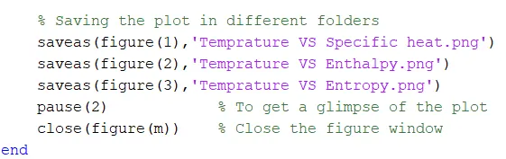
- end is used to end the loop.
- Step 20:
- To print the molecular weight of every species, the following lines have been written.
- n{m}, t{m} collects the species name from the data file, then we convert the row matrix to column matrix to create a simpler looking array.
- Then we call the function Molecular_weight to calculate and display the value in the command window.
- n{m}, t{m} collects the species name from the data file, then we convert the row matrix to column matrix to create a simpler looking array.

- Printed molecular weight in command window is as below
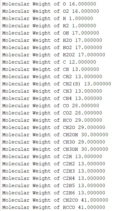
- To print the molecular weight of every species, the following lines have been written.
- Step 21:
-
function w=Molecular_weight(t) atomic_name=['H' 'C' 'O' 'N' 'Ar']; % Atomic name array atomic_weight=[1 12 16 14 40]; % Atomic weight array w=0; % To clear last iteration value for i=1:length(t) for j=1:length(atomic_name) if strcmp(t(i),atomic_name(j)) % Comparing species characters and atomic_name array w=w+atomic_weight(j); % Calculating atomic weight position=j; % Creating new variable to store value of j after the loop end end n=str2num(t); % Converting string to number if n>1 w=w+atomic_weight(position)*(n-1); % Calculating molecular weight end end fprintf('Molecular Weight of %s ',t); % Displaying molecular weight fprintf('%f \n',w); % Displaying new line disp('') % Displaying above lines end- The first step is to define the function handle(Molecular_weight), input(t), and output(w).
- An array of atomic_name has been defined consisting of H, C, O, N, and Ar.
- In a similar way, atomic_weight array has been defined which consists of the molecular weight of the respective atoms.
- The next step is to start with zero molecular weight.
- The logic starts with a for loop, iterations are the length of species characters than, other for-loop checks with atomic_name array. To compare strcmp command is used.
- If the strcmp returns a true value then we take the molecular weight of that corresponding atom and use it to calculate the molecular weight.
- For more than one atom in a molecule, we calculate the number of atoms and then calculate the molecular weight of corresponding atoms.
- To display the molecular weight value we use the fprintf and disp command.
-
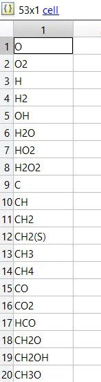
- Screenshot of the window where all the folders are saved.
-
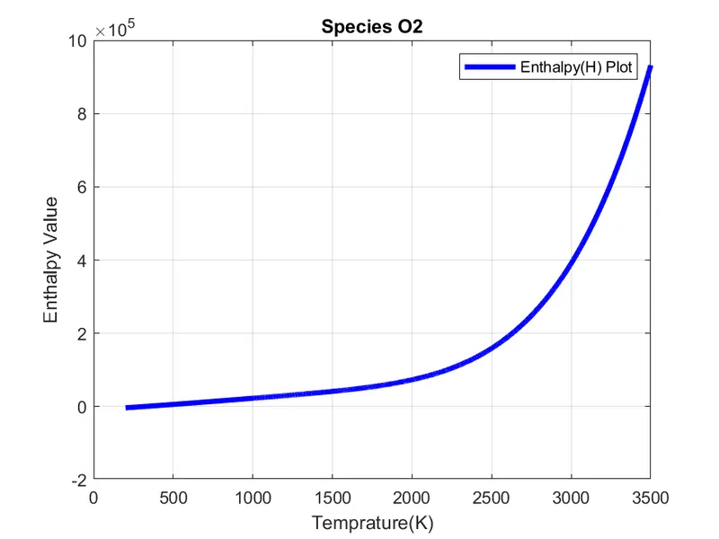
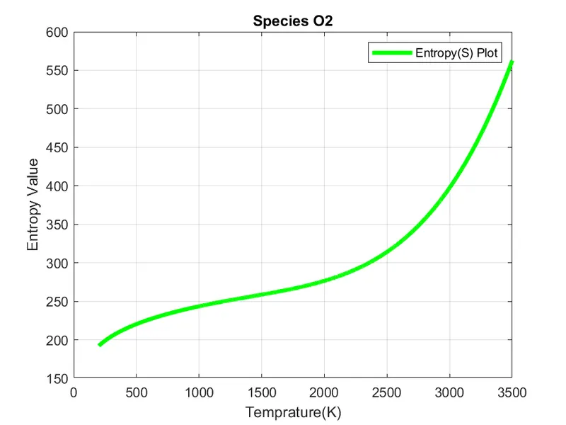
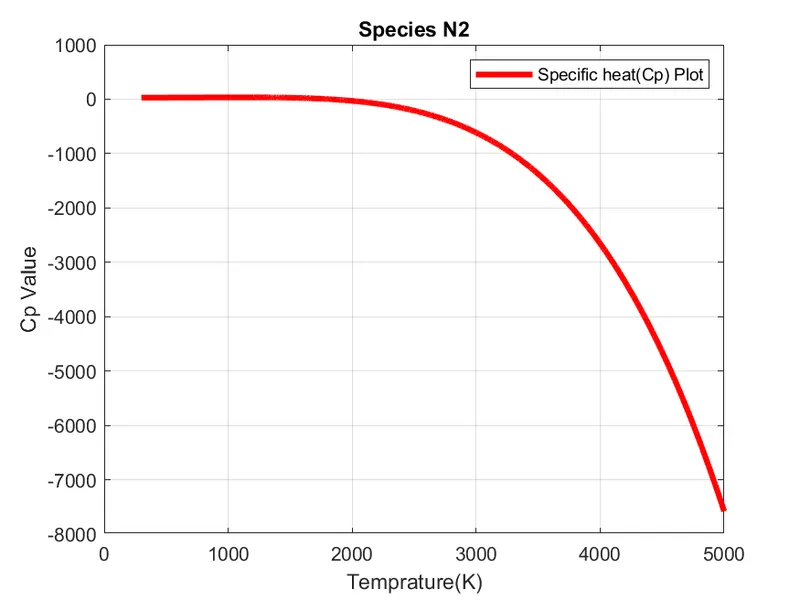
- Plots for O2, N2, and Co2 species (your program should be case insensitive if it is going to take the species name as an input).
- Plots for O2:
- Enthalpy(H) Plot
- Entropy(S) Plot
- Specific heat (Cp) Plot
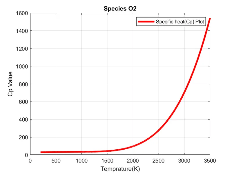
- Enthalpy(H) Plot
- Plots for N2:
- Enthalpy(H) Plot
- Entropy (S) Plot
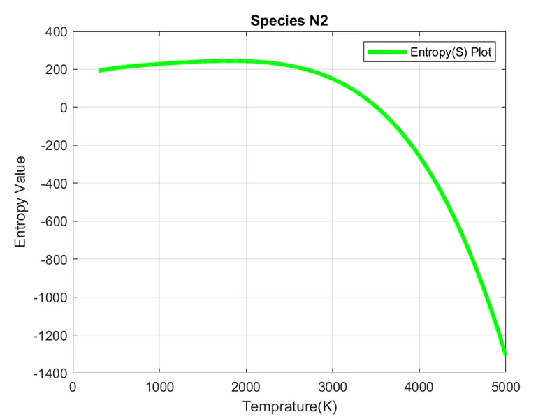
- Specific heat(Cp) Plot
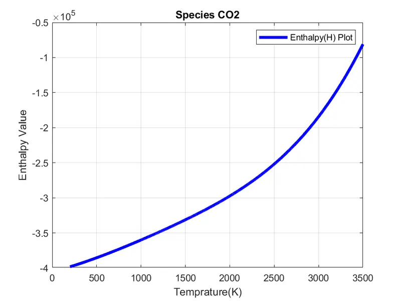
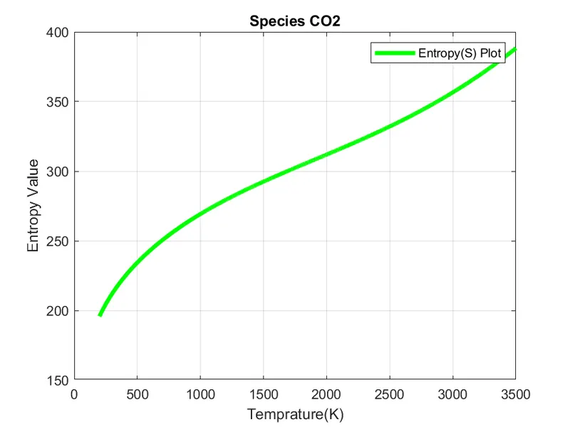
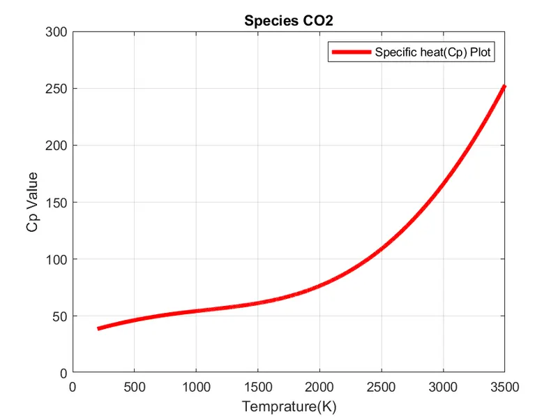
- Plots for CO2:
- Enthalpy(H) Plot
- Entropy(S) Plot
- Specific(Cp) Plot
- Plots for O2:
Errors
- Faced problem while coding the subject overcame by taking different iterations.
- Still have some problems while coding the molecular weight. Can't able to capture the number in strings of species of molecules.
- Tried to overcome it but didn't able to overcome it.
- While saving the plots in another directory I faced problems in syntax so I took reference from other reports and Matlab documentation.
References