Parsing NASA thermodynamic data using MATLAB

Parsing of NASA's thermodynamic data using MATLAB

Parsing of a file means reading inputs in the form of a data file, and storing this data.

NASA has created a data file called THERMO.dat, which contains detailed information about 53 different species, and their coefficients.

These coefficients can be used to obtain meaningful thermodynamic properties, namely: Specific Heat, Enthalpy, and Entropy.

From the data file, the first 7 coefficients are low temperature coefficents, whereas the next 7 are high temperature coefficients.

R is the universal gas constant, 8.314 J/mol-K

Temperatures are in K

Cp represents the specific heat (J/kg-K), H the enthalpy (J/mol), and S the entropy. (J/K).

A snip of the dat file:

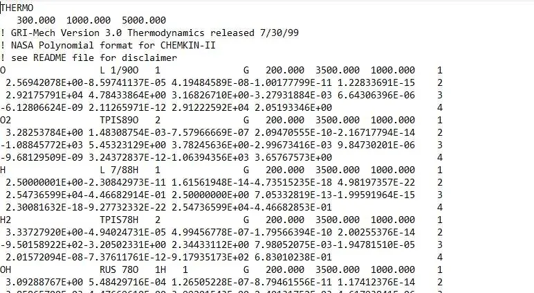
In this project, the dat file from NASA is parsed using MATLAB to obtain all the coefficients.

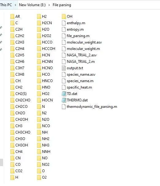
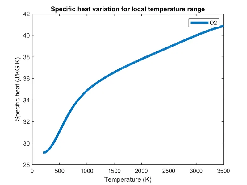
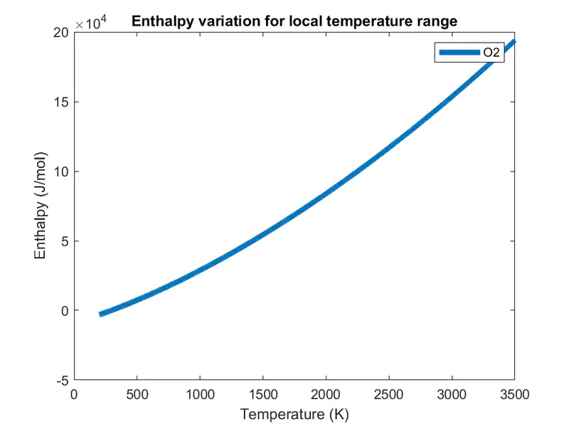
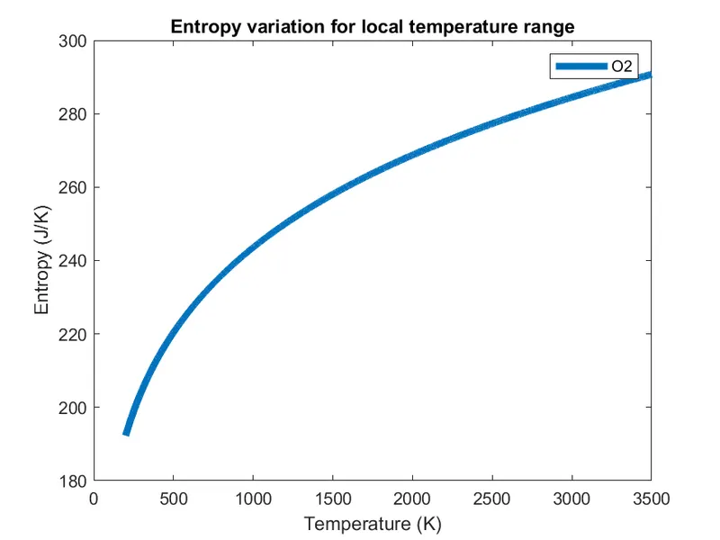
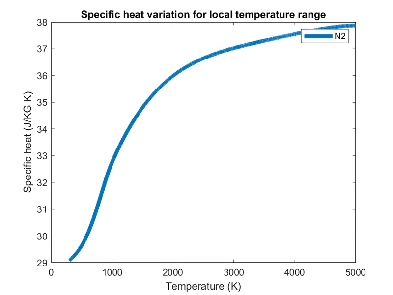
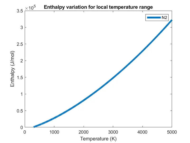
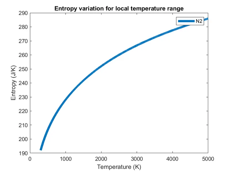
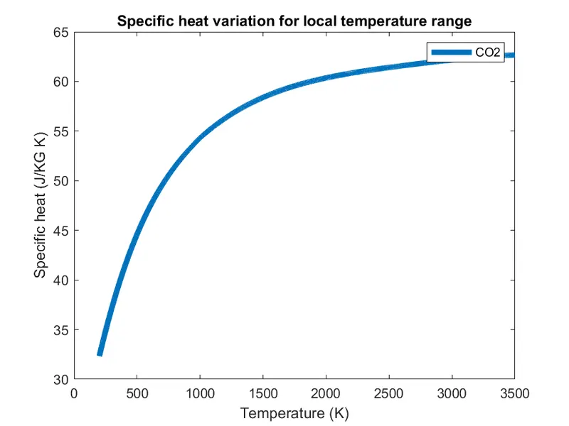
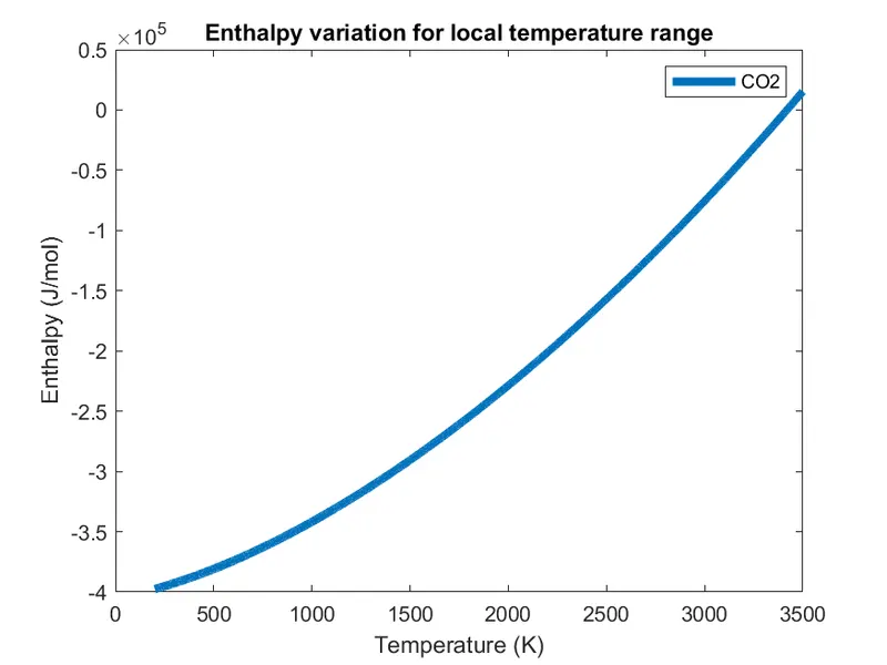
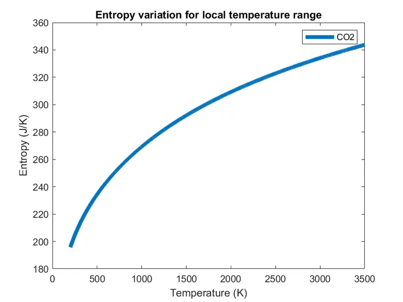
Next, each coefficient's enthalpy, entropy, and specific heats are calculated, and the plots of local temperature variation vs these thermodynamic properties are saved in new folders.

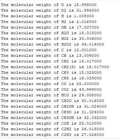
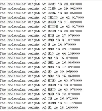
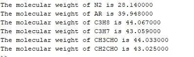
Molecular weights of each species are calculated as well.

Note: The file THERMO.dat has been copied, saved as TD.dat and then used for parsing to prevent any unexpected changes to the original file.

Seperate functions are created for the thermodynamic properties and the molecular weight.

Code for the main program:

close all 
clear all
clc

f1 = fopen('TD.dat','r');
fgetl(f1); %reads 'Thermo'

% extracting the global temperatures
temp_rangeline = fgetl(f1); %this is a string
split = strsplit(temp_rangeline,' '); %splits at each delimiter (' ')
temp_global_lower = str2double(split{2});
temp_global_mid = str2double(split{3});
temp_global_higher = str2double(split{4});

%skipping the comments after global temperature line
A = fgetl(f1);
B = fgetl(f1);
C = fgetl(f1);

%inputs
num_species = 53;
R = 8.314;


%species block
for i = 1:num_species
  species_line = fgetl(f1); %species heading
  
  %extracting the local temperature ranges
  split_species_name = strsplit(species_line,' '); 
  species_name = split_species_name{1};
  
  G_loc = strfind(species_line,'G');
  temp_local_lowerstr = species_line(G_loc+4:G_loc+10);
  temp_local_lower = str2double(temp_local_lowerstr);
   
  temp_local_higherstr = species_line(G_loc+13:G_loc+20);
  temp_local_higher = str2double(temp_local_higherstr);
  
  temp_local_midstr = species_line(G_loc+22:G_loc+30);
  temp_local_mid = str2double(temp_local_midstr);
 
  x = temp_local_lower;
  y = temp_local_mid;
  z= temp_local_higher;
  
  %extracting the species block
  line2 = fgetl(f1);
  e_loc = strfind(line2,'E');
  
  %high temperature coefficients
  a1str = line2(1:e_loc(1)+3);
  a1 = str2double(a1str);
  
  a2str = line2(e_loc(1)+4:e_loc(2)+3);
  a2= str2double(a2str);
  
  a3str = line2(e_loc(2)+4:e_loc(3)+3);
  a3 = str2double(a3str);
  
  a4str = line2(e_loc(3)+4:e_loc(4)+3);
  a4 = str2double(a4str);
  
  a5str = line2(e_loc(4)+4:e_loc(5)+3);
  a5 = str2double(a5str);
  
  line3 = fgetl(f1);
  e_loc = strfind(line3,'E');
  
  a6str = line3(1:e_loc(1)+3);
  a6 = str2double(a6str);
  
  a7str = line3(e_loc(1)+4:e_loc(2)+3);
  a7 = str2double(a7str);
  
  %low temperature coefficients
  b1str = line3(e_loc(2)+4:e_loc(3)+3);
  b1 = str2double(b1str);
  
  b2str = line3(e_loc(3)+4:e_loc(4)+3);
  b2 = str2double(b2str);
  
  b3str = line3(e_loc(4)+4:e_loc(5)+3);
  b3 = str2double(b3str);
  
  line4 = fgetl(f1);
  e_loc = strfind(line4,'E');
  
  b4str = line4(1:e_loc(1)+3);
  b4 = str2double(b4str);
  
  b5str = line4(e_loc(1)+4:e_loc(2)+3);
  b5 = str2double(b5str);
  
  b6str = line4(e_loc(2)+4:e_loc(3)+3);
  b6 = str2double(b6str);
  
  b7str = line4(e_loc(3)+4:e_loc(4)+3);
  b7 = str2double(b7str);
  
  temp_range = (x:z); 
  
%thermodynamic properties
[cp] = specific_heat(x,y,z,a1,a2,a3,a4,a5,b1,b2,b3,b4,b5,R,temp_range);
[h] = enthalpy(x,y,z,a1,a2,a3,a4,a5,a6,a7,b1,b2,b3,b4,b5,b6,b7,R,temp_range);
[s] = entropy(x,y,z,a1,a2,a3,a4,a5,a6,a7,b1,b2,b3,b4,b5,b6,b7,R,temp_range);

mw = molecular_weight(species_name);
mm = sprintf('The molecular weight of %s is %f',species_name,mw);
disp(mm)


foldername = sprintf('%s',species_name);
mkdir(foldername)
figure(1)
   plot(temp_range,cp,'linewidth',4);
   xlabel('Temperature (K)')
   ylabel('Specific heat (J/KG K)')
   title('Specific heat variation for local temperature range') 
   legend(species_name)
   picturename1 = fullfile(foldername,'Cp vs T');
   saveas(gcf,picturename1,'png')
   
   
figure(2)
   H_vs_temperature = plot(temp_range,h,'linewidth',4);
   xlabel('Temperature (K)')
   ylabel('Enthalpy (J/mol)')
   title('Enthalpy variation for local temperature range')
   legend(species_name)
   picturename2 = fullfile(foldername,'H vs T');
   saveas(gcf,picturename2,'png')
   
figure(3)
   S_vs_temperature = plot(temp_range,s,'linewidth',4);
   xlabel('Temperature (K)')
   ylabel('Entropy (J/K)')
   title('Entropy variation for local temperature range')
   legend(species_name)
   picturename3 = fullfile(foldername,'S vs T');
   saveas(gcf,picturename3,'png')

end

Basic steps:

1. The file is first open using fopen and stored in a pointer to the file, f1.
2. The first few lines are comments, and thus are skipped using fgetl command, which moves a line forward.
3. The global temperature line is extracted and stored, although it is not used.
4. To extract the global temperatures, first the temperature line is stored in an array, which is then split using strsplit, as explained in the comments.
5. str2double converts each string of the string that has been split into a number, which is stored in a variable.
6. The next few comments are skipped using fgetl, and finally the species block is parsed.
7. There are 53 species, and thus a for loop is run 53 times to ensure each species block is parsed.
8. For each species, the parsing procedure is simple: extract the species name, and local temperature ranges for each species similar to steps 3 - 5.
9. Use fgetl to move to a coefficient line, convert the string to a number using str2double.
10. Call the functions described further in this report, and create + save the plots in new folders specific to each species.
11. The mkdir command is used to make a new folder for each species, thus creating a new folder each loop.
12. fullfile and saveas are used to save the plots as images.

It can be noted that 4 functions are called.

These are as follows:

Specific heat

                               
function [cp] = specific_heat(x,y,z,a1,a2,a3,a4,a5,b1,b2,b3,b4,b5,R,temp_range)
for j = 1:length(temp_range)
    T(j) = temp_range(j);
      if T(j)

An if else switch case is used to seperate the low and high temperature coefficients. y is the mid range temperature, and thus for any temperature below this, the low temperature coefficients are used, else the high temperature.

The same logic applies to the enthalpy and entropy.

Enthalpy

function [h] = enthalpy(x,y,z,a1,a2,a3,a4,a5,a6,a7,b1,b2,b3,b4,b5,b6,b7,R,temp_range)
for j = 1:length(temp_range)
    T(j) = temp_range(j);
    if T(j)

Entropy

function [s] = entropy(x,y,z,a1,a2,a3,a4,a5,a6,a7,b1,b2,b3,b4,b5,b6,b7,R,temp_range)
for j = 1:length(temp_range)
    T(j) = temp_range(j);
    if T(j)

For molecular weight

function [mw] = molecular_weight(species_name)
 
 atomic_mass = [15.999, 1.008, 12.001, 14.07, 39.948];
 elements = ['O', 'H', 'C', 'N', 'A'];
 
 m_wt = 0;
 for i= 1:length(species_name)
     for j = 1:length(elements)
         %if starts
         if strcmp(species_name(i),elements(j))
             m_wt = m_wt + atomic_mass(j);
             position = j;
         end
         %if ends
     end
  n = str2double(species_name(i));
  if (n>1)
      m_wt = m_wt + atomic_mass(position)*(n-1);
  end
 end
 mw = m_wt;
 end

Molecular weights of all the species:

The folder where all the plots have been saved:

Plots for O2, N2 and CO2 Species

O2

N2

CO2

Conclusion

MATLAB is an efficient interface that allows ease of file parsing. In a short span of time, the NASA's thermodynamic file has been parsed to obtain multiple meaningful thermodynamic data which can be used for further important studies.

References

MATLAB documentation