Parsing NASA thermodynamic data

A: NASA proposed thermodynamic data which contains coefficients of functions of specific heat at constant pressure, enthalpy and entropy. The data file is used to calculate thermodynamic properties.

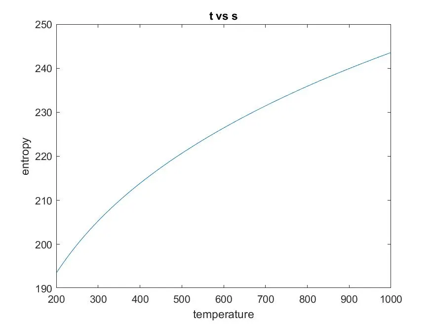
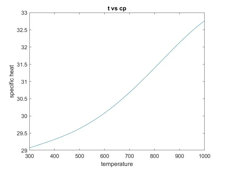
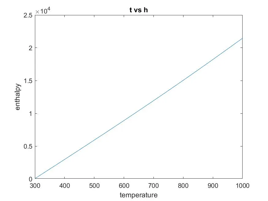
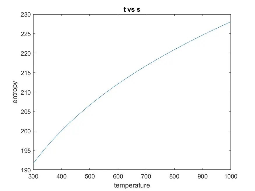
Aim: To calculate the thermodynamic properties like specific heat, enthalpy and entropy by parsing the data, proposed by NASA and plotting the variations against the temperature of these thermal properties. To find the molecular masses of these species and storing the output in a separate folder. The whole process is done in MATLAB.

Data file: NASA thermodynamic data

Theory:

File parsing: The process of "parsing" can be described as reading in a data stream of some sort and building an in-memory model or representation of the semantic content of that data, to facilitate performing some kind of transformation on the data.

Formulas for finding three thermal properties:

Terms used in code:

• a1 to a14 = coefficients of thermal properties.
• R = Universal gas constant = 8.314.
• t = variable used for calculation in local temperature ranges.
  
  
• lt1 = local low temperature.
  
  
• lt2 = local mid temperature.
  
  
• lt3 = local high temperature.
  
  
• cp = specific heat.
  
  
• h = enthalpy.
  
  
• s = entropy.
  
  
• AW = atomic weight.

Function code and explanation:

1. In this code, we give input values of all coefficients and temperatures.
   
   
2. Open the new script and add function with tvalues name. Since we are calculating three properties, we give three output variables i.e., fv1, fv2, fv3.
   
   function [fv1, fv2, fv3] = tvalues(a1, a2, a3, a4, a5, a6, a7, t, lt2, a8, a9, a10, a11, a12, a13, a14)
   
   
3. We know universal gas constant value is 8.314 which is given to a variable called R.
   
   R = 8.314;
   
   
4. We know that temperatures are from low to high. Coefficients are substituted in formulas in two types. If the temperature is more than local mid-temperature, a1 to a7 coefficients are used for calculation. If the temperature is less than local mid-temperature, a8 to a14 coefficients are used for calculation. This can be done by if-else statements. The formula is expressed interest of specific heat, enthalpy and entropy.
   
   if t > lt2
   fv1 = R * (a1 + (a2 * t) + (a3 * (t).^2) + (a4 * (t).^3) + (a5 * (t).^4));
   fv2 = R * t .* (a1 + ((a2 * t)./2) + ((a3 * (t).^2)/3) + ((a4 * (t).^3)/4) + ((a5 * (t).^4)/5) + (a6./t));
   fv3 = R * ((a1 * log(t)) + (a2 * t) + ((a3 * (t).^2)/2) + ((a4 * (t).^3)/3) + ((a5 * (t).^4)/4) + a7);
   
   
5. else statement is used for other temperatures.
   
   else
   fv1 = R * (a8 + (a9 * t) + (a10 * (t).^2) + (a11 * (t).^3) + (a12 * (t).^4));
   fv2 = R * t .* (a8 + ((a9 * t)./2) + ((a10 * (t).^2)/3) + ((a11 * (t).^3)/4) + ((a12 * (t).^4)/5) + (a13./t));
   fv3 = R * ((a8 * log(t)) + (a9 * t) + ((a10 * (t).^2)/2) + ((a11 * (t).^3)/3) + ((a12 * (t).^4)/4) + a14);
   
   
6. Close the function with end command.
   
   end
   
   
7. Save the function script in the name of a function.

Function code:

function [fv1, fv2, fv3] = tvalues(a1, a2, a3, a4, a5, a6, a7, t, lt2, a8, a9, a10, a11, a12, a13, a14)

R = 8.314;

if t > lt2
    fv1 = R * (a1 + (a2 * t) + (a3 * (t).^2) + (a4 * (t).^3) + (a5 * (t).^4));
    fv2 = R * t .* (a1 + ((a2 * t)./2) + ((a3 * (t).^2)/3) + ((a4 * (t).^3)/4) + ((a5 * (t).^4)/5) + (a6./t));
    fv3 = R * ((a1 * log(t)) + (a2 * t) + ((a3 * (t).^2)/2) + ((a4 * (t).^3)/3) + ((a5 * (t).^4)/4) + a7);

else
    fv1 = R * (a8 + (a9 * t) + (a10 * (t).^2) + (a11 * (t).^3) + (a12 * (t).^4));
    fv2 = R * t .* (a8 + ((a9 * t)./2) + ((a10 * (t).^2)/3) + ((a11 * (t).^3)/4) + ((a12 * (t).^4)/5) + (a13./t));
    fv3 = R * ((a8 * log(t)) + (a9 * t) + ((a10 * (t).^2)/2) + ((a11 * (t).^3)/3) + ((a12 * (t).^4)/4) + a14);
end

Code procedure and explanation:

1. Add statements as shown below.
   
   clear all
   close all
   clc
   
   
2. First, we need to open the data file. To open the data file, we use fopen command in reading mode. The file is assigned to a variable called fp. Make sure that data file is in the same directory of MATLAB current running program.
   
   fp = fopen('thermo.dat', 'r')
   
   
3. Now, we need to read the data which can be done by the command fgetl. It is a command which reads the data line by line and every time we run it, we get next line. The file contains a header and we give name as the heading variable.
   
   heading = fgetl(fp)
   
   
4. Next line contains global temperatures of species. These are extracted by fgetl command. This is assigned to a gbt variable.
   
   gbt = fgetl(fp)
   
   
5. The output is in string format. We need to split the string and convert them into numbers. Splitting is done by strsplit and converting can be done by str2num commands.
   
   gts = strsplit(gbt, ' ')
   
   for i = 1 : length(gts)
   gt{i} = str2num(gts{i})
   end
   
   
6. Assigning global temperatures.
   
   global_low_temp = gt{2}
   global_mid_temp = gt{3}
   global_high_temp = gt{4}
   
   
7. Next three lines are comments which can be neglected and drawn by fgetl command.
   
   c1 = fgetl(fp);
   c2 = fgetl(fp);
   c3 = fgetl(fp);
   
   
8. The header is extracted and there are 53 species in the data. We can observe that each data consists of coefficient values are represented in the four lines. By applying logic we can extract these coefficients for calculating thermal properties.
   
   for ce 1 : 53
   ls = fgetl(fp);
   l1 = strsplit(ls, ' ')
   species = l1{1}
   
   lt1 = str2num(l1{end - 3})
   lt2 = str2num(l1{end - 2})
   lt3 = str2num(l1{end - 1})
   
   
9. We got local temperatures for the species. These are the temperatures which are used for calculation. The temperature range can be given as follows.
   
   t = linspace(lt1, lt2, 100);
   
   
10. There are three lines of coefficients in the data file. The values are represented in the power of 'E'. These values are extracted by finding the string 'E' positions and converted into numbers.
    
    ls1 = fgetl(fp);
    l2 = strfind(ls1, 'E');
    
    a1 = str2num(ls1(1 : l2(1)+3));
    a2 = str2num(ls1(l2(1)+4 : l2(2)+3));
    a3 = str2num(ls1(l2(2)+4 : l2(3)+3));
    a4 = str2num(ls1(l2(3)+4 : l2(4)+3));
    a5 = str2num(ls1(l2(4)+4 : l2(5)+3));
    
    
11. Till now, we got coefficients from the second line and we need to extract from the third and fourth lines. The coefficients are represented from a1 to a14. Next coefficients are also found in the same manner.
    
    ls2 = fgetl(fp);
    l3 = strfind(ls2, 'E');
    
    a6 = str2num(ls2(1 : l3(1)+3));
    a7 = str2num(ls2(l3(1)+4 : l3(2)+3));
    a8 = str2num(ls2(l3(2)+4 : l3(3)+3));
    a9 = str2num(ls2(l3(3)+4 : l3(4)+3));
    a10 = str2num(ls2(l3(4)+4 : l3(5)+3));
    
    ls3 = fgetl(fp);
    l4 = strfind(ls3, 'E');
    
    a11 = str2num(ls3(1 : l4(1)+3));
    a12 = str2num(ls3(l4(1)+4 : l4(2)+3));
    a13 = str2num(ls3(l4(2)+4 : l4(3)+3));
    a14 = str2num(ls3(l4(3)+4 : l4(4)+3));
    
    
12. We got all 14 values of coefficients for all 53 species. Now we need to calculate the values of specific heat, enthalpy and entropy. We know that temperature higher than lt2, have coefficients from a1 to a7 and a temperature lower than lt2 have coefficients a8 to a14.
    
    
13. The formulas for specific heat, enthalpy and entropy are given in another script. Here we call the function and perform calculations.
    
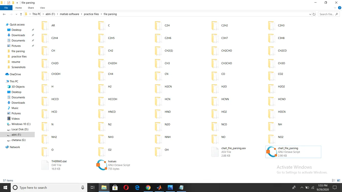
    [cp, h, s] = values(a1, a2, a3, a4, a5, a6, a7, t, lt2, a8, a9, a10, a11, a12, a13, a14)
    
    
14. Therefore, we got values of thermal properties. We should plot the graphs of these thermal properties individually against respective local temperatures. Since we get three plots for each species, we can't find the respective plot in the file directory. To avoid confusion, we create folders for plots of the respective species and store them in a very well manner.
    
    
15. Creating a folder in the current directory can be done by the command mkdir. This creates a separate folder for each species and stores the plot in it. We are creating in the name of species.
    
    mkdir(species)
    
    
16. We know that MATLAB process runs in a particular directory. To store the plots in the species folder, we need to change the directory. Changing can be done by using another command cd.
    
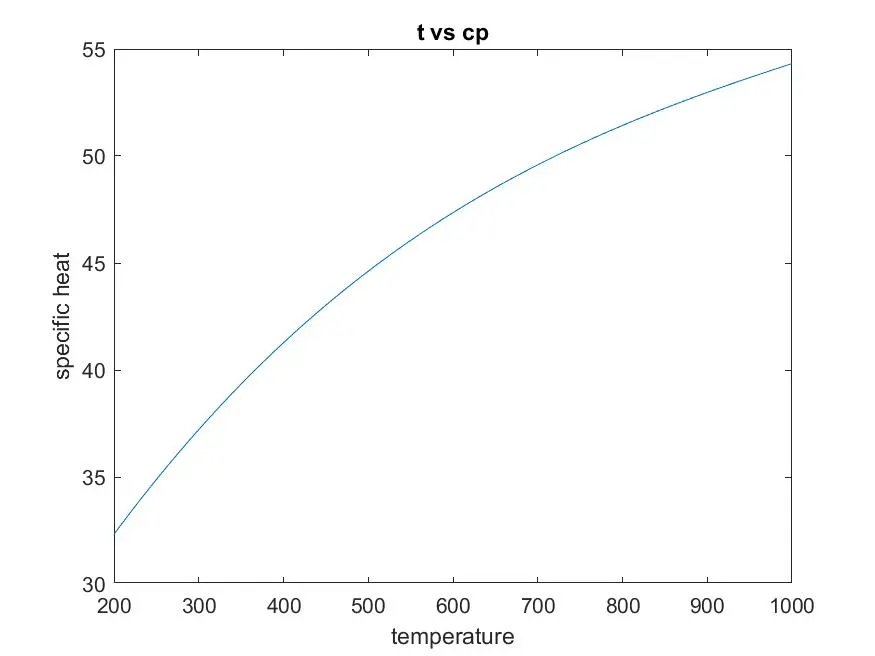
    cd(species)
    
    
17. We should plot three figures of specific heat, enthalpy and entropy against temperature. Three figures are plotted separately. Plotting graphs and labelling them are done.
    
    figure(1)
    plot(t, cp)
    xlabel('temperature')
    ylabel('specific heat')
    title('t vs cp')
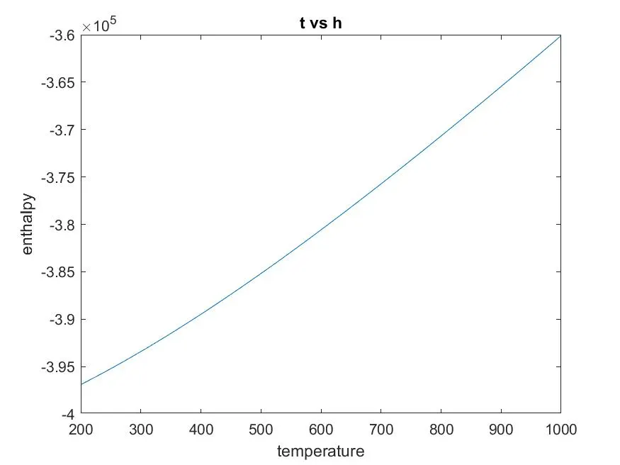
    saveas(gcf, 't_vs_cp.jpg')
    
    
18. Same commands are used for second and third figures.
    
    figure(2)
    plot(t, h)
    xlabel('temperature')
    ylabel('enthalpy')
    title('t vs h')
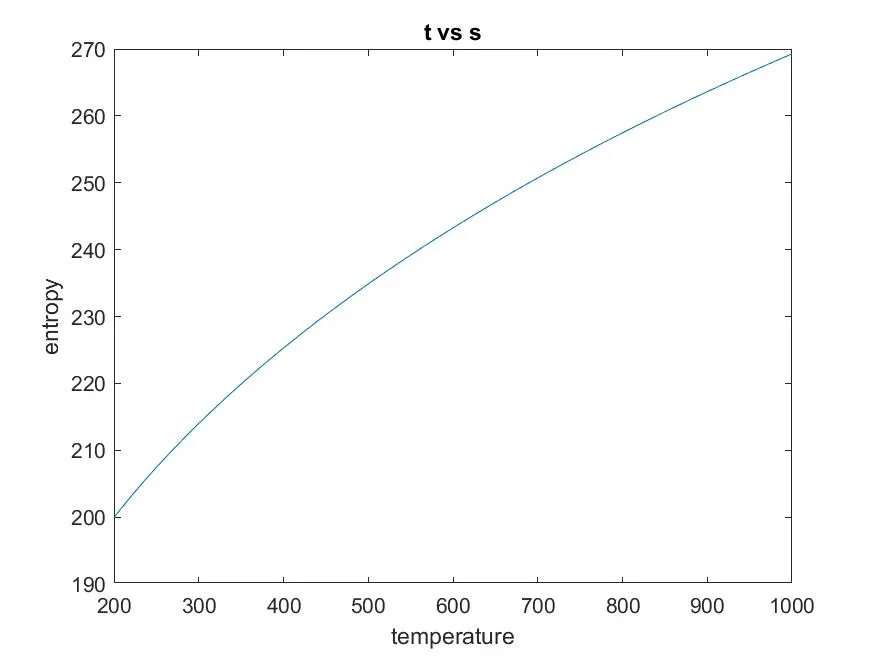
    saveas(gcf, 't_vs_h.jpg')
    
    figure(3)
    plot(t, s)
    xlabel('temperature')
    ylabel('entropy')
    title('t vs s')
    saveas(gcf, 't_vs_s.jpg')
    
    
19. The plots are saved in species folder in the format of .jpg. Since the program should run in the previous directory, we need to change the running program into the previous directory. This can be done by using command cd../.
    
    cd../
    
    
20. Till now, we solved values of each thermal properties and also plots are generated of these properties against temperature in separate folders.
    
    
21. We should calculate each species molecular weight. This can be done by the following code.
    
    
22. Initially, species atomic names are assigned.
    
    s_atomic_name = {'H', 'C', 'N', 'O', 'AR'};
    
    
23. Now, we should give the atomic weights.
    
    AW = [1 12 14 16 40];
    
    
24. Initially, the weight value is given as zero for counter loops.
    
    W = 0;
    
    
25. Add for loops with counter variables for q and p with lengths of species name and s_atomic_name.
    
    for p = 1 : length(species)
    for q = 1 : length(s_atomic_name)
    
    
26. Add if statements for comparing two strings. Two strings are species name and s_atomic_name.
    
    if strcmp(species(p), s_atomic_name(q)) == 1
    
    
27. Add weight W counter with atomic weight AW.
    
    W = W + AW(p);
    
    
28. Position variable value is assigned with q.
    
    position = q;
    
    
29. End the if statement with end command.
    
    end
    
    End the if statement with end command.
    
    end
    
    
30. The string is converted to num by using command 'str2double' with n variable.
    
    n = str2double(species(p));
    
    
31. Add if statement and weights are calculated and end it. The statement should be written in such a way that, left and right sides should be the same number of elements.
    
    if n>1
    W = W + ((AW(position)) * (n - 1));
    end
    
    
32. End one loop.
    
    end
    
    
33. Display molecular weights with the species name.
    
    molecular_weight = sprintf('%s, %f',species, W)
    
34. End the final loop.
    
    end

Code:

clear all
close all
clc

% File opening
fp = fopen('thermo.dat', 'r');

% Extracting header
heading = fgetl(fp);

% global temperatues
gbt = fgetl(fp);
gts = strsplit(gbt, ' ');

for i = 1 : length(gts)
    gt{i} = str2num(gts{i});
end
% assigning global tempeartues
gloabl_low_temp = gt{2};
gloabl_mid_temp = gt{3};
gloabl_high_temp = gt{4};

% extracting comments
c1 = fgetl(fp);
c2 = fgetl(fp);
c3 = fgetl(fp);

% Extracting coefficients

for ce = 1 : 53
    
    
    ls = fgetl(fp);
    l1 = strsplit(ls, ' ');
    species = l1{1};
    
    lt1 = str2num(l1{end-3});
    lt2 = str2num(l1{end-2});
    lt3 = str2num(l1{end-1});
    
    t = linspace(lt1, lt3, 100);
    
    % Extracting line 2
    
    ls1 = fgetl(fp);
    l2 = strfind(ls1, 'E');
    
    a1 = str2num(ls1(1 : l2(1)+3));
    a2 = str2num(ls1(l2(1)+4 : l2(2)+3));
    a3 = str2num(ls1(l2(2)+4 : l2(3)+3));
    a4 = str2num(ls1(l2(3)+4 : l2(4)+3));
    a5 = str2num(ls1(l2(4)+4 : l2(5)+3));
    
    % Extracting line 3    
    ls2 = fgetl(fp);
    l3 = strfind(ls2, 'E');
    
    a6 = str2num(ls2(1 : l3(1)+3));
    a7 = str2num(ls2(l3(1)+4 : l3(2)+3));
    a8 = str2num(ls2(l3(2)+4 : l3(3)+3));
    a9 = str2num(ls2(l3(3)+4 : l3(4)+3));
    a10 = str2num(ls2(l3(4)+4 : l3(5)+3));
    
    % Extracting line 4
    
    ls3 = fgetl(fp);
    l4 = strfind(ls3, 'E');
    
    a11 = str2num(ls3(1 : l4(1)+3));
    a12 = str2num(ls3(l4(1)+4 : l4(2)+3));
    a13 = str2num(ls3(l4(2)+4 : l4(3)+3));
    a14 = str2num(ls3(l4(3)+4 : l4(4)+3));
    
    % Calculating thermal properties values
    
    [cp, h, s] = tvalues(a1,a2,a3,a4,a5,a6,a7,t,lt2,a8,a9,a10,a11,a12,a13,a14);
    
    % creating folder
    mkdir(species)
    
    % changing directory
    cd(species)
    
    % plots are generated and saved in separate folder
    figure(1)
    plot(t,cp)
    xlabel('temperature')
    ylabel('specific heat')
    title('t vs cp')
    saveas(gcf, 't_vs_cp.jpg')
    
    figure(2)
    plot(t,h)
    xlabel('temperature')
    ylabel('enthalpy')
    title('t vs h')
    saveas(gcf, 't_vs_h.jpg')
    
    figure(3)
    plot(t,s)
    xlabel('temperature')
    ylabel('entropy')
    title('t vs s')
    saveas(gcf, 't_vs_s.jpg')
    
    % changing folder to the previous folder
    cd ../
    
    % calculating molecular weights
    s_atomic_name = {'H','C','N','O','AR'};
    AW = [1 12 14 16 40];
    W = 0;

    
    for p = 1 : length(species)
        for q = 1 : length(s_atomic_name)
            % comparing with strings
            if strcmp(species(p), s_atomic_name(q)) == 1
                W = W + AW(q);
                position = q;
            end
        end
        n = str2double(species(p));
        if n > 1
            % finding weights
            W = W + ((AW(position)) * (n - 1));
        end
    end
    molecular_weight = sprintf('%s, %f',species, W)
end

Output in the command window:

Values of molecular weight are shown in the command window.

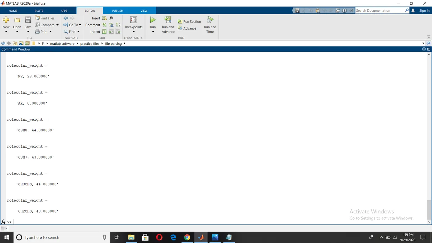
Final values in a workspace:

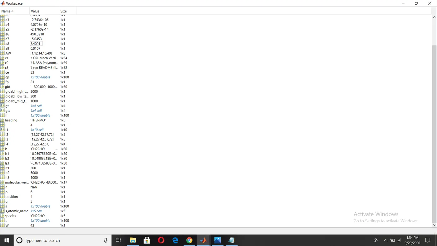
Plots generated:

O2:

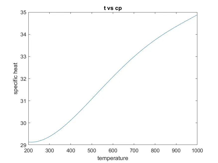
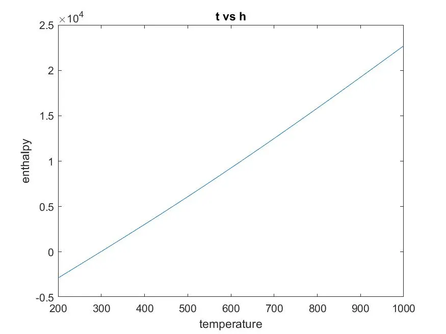
N2:

CO2:

Folders created in the file manager:

Points to remember:

• The data file should be in the same directory for opening the file.
  
  
• The logic should be applied in the code correctly while extracting coefficients.
  
  
• fgetl is a command which is used for extracting data line by line. Each time we use it, the next line is extracted.
  
  
• str2num is a command which is used to convert from string to number.
  
  
• strfind is used to find a particular string.
  
  
• mkdir is used to create a folder and cd.. is used to change the running program into a different folder.

Errors occurred:

1. An error occurred while converting a string to a number. An error occurred when '()' are used. We should use '{}' instead of '()'.
   
   Wrong: gt{i} = str2num(gts(i));
   Correct: gt{i} = str2num(gts{i});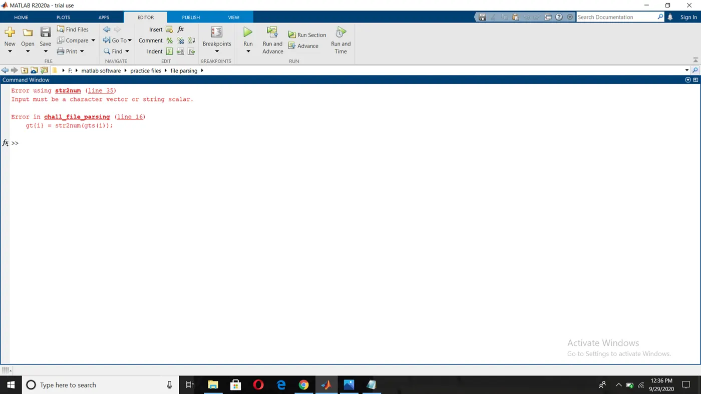
   
   
   
   

Conclusion: Hence, by using MATLAB, coefficients are extracted from the data file proposed by NASA. Values of thermal properties are calculated in their respective temperature ranges. Plots are created for all species of specific heat, enthalpy and entropy against respective local temperature range. Each plot is created in species folder. Molecular weights are calculated for all species.