Project 1 - Data Handling and Interpolation

Project 1:

MATLAB CODE:

% Define the function for simple harmonic oscillator

function dxdt = harmonic_oscillator(t, x, m, k)

dxdt = zeros(2,1);

dxdt(1) = x(2);

dxdt(2) = - (k/m) * x(1);

end

% Input dialog box to get 'm' and 'k' values from user

prompt = {'Enter mass m:', 'Enter spring constant k:'};

dlgtitle = 'Input';

dims = [1 35]; % Dimensions of the input dialog box

definput = {'1', '1'}; % Default input values

answer = inputdlg(prompt, dlgtitle, dims, definput);

m = str2double(answer{1});

k = str2double(answer{2});

% Initial conditions

x0 = [1; 0]; % Assuming Initial displacement and velocity values

% Time span

tspan = [0 10];

% Solve using ode45

[t_ode45, x_ode45] = ode45(@(t, x) harmonic_oscillator(t, x, m, k), tspan, x0);

% Solve using ode23

[t_ode23, x_ode23] = ode23(@(t, x) harmonic_oscillator(t, x, m, k), tspan, x0);

% Plot results for ode45

figure;

subplot(3, 1, 1);

plot(t_ode45, x_ode45(:, 1), 'b', 'LineWidth', 1.5);

title('ODE45 Solution');

xlabel('Time (s)');

ylabel('Displacement x');

grid on;

subplot(3, 1, 2);

plot(t_ode45, x_ode45(:, 2), 'r', 'LineWidth', 1.5);

title('ODE45 Solution');

xlabel('Time (s)');

ylabel('Velocity x\_dot');

grid on;

subplot(3, 1, 3);

plot(t_ode45, - (k/m) * x_ode45(:, 1), 'g', 'LineWidth', 1.5);

title('ODE45 Solution');

xlabel('Time (s)');

ylabel('Acceleration x\_dot\_dot');

grid on;

% Plot results for ode23

figure;

subplot(3, 1, 1);

plot(t_ode23, x_ode23(:, 1), 'b', 'LineWidth', 1.5);

title('ODE23 Solution');

xlabel('Time (s)');

ylabel('Displacement x');

grid on;

subplot(3, 1, 2);

plot(t_ode23, x_ode23(:, 2), 'r', 'LineWidth', 1.5);

title('ODE23 Solution');

xlabel('Time (s)');

ylabel('Velocity x\_dot');

grid on;

subplot(3, 1, 3);

plot(t_ode23, - (k/m) * x_ode23(:, 1), 'g', 'LineWidth', 1.5);

title('ODE23 Solution');

xlabel('Time (s)');

ylabel('Acceleration x\_dot\_dot');

grid on;

Explanation:

harmonic_oscillator Function: This function defines the system of differential equations for the simple harmonic oscillator. It takes time t, state vector x, mass m, and spring constant k as inputs and the output is dxdt, which is a vector containing the derivatives:

dxdt(1) which is the velocity (dx/dt = v).

dxdt(2) which is the acceleration (dv/dt = -k/m * x).

Input Dialog Box: This part prompts the user to enter the values for the mass m and the spring constant k using an input dialog box. The values entered are converted from strings to numeric values using str2double.

Initial Conditions: x0 = [1; 0] sets the initial position to 1 and the initial velocity to 0.

Time Span: tspan = [0 10] specifies the time interval for the simulation, from 0 to 10 seconds.

ode45 and ode23 are numerical solvers for ordinary differential equations.

ode45 is a higher-order Runge-Kutta method, while ode23 is a lower-order method, so ode45 generally provides better accuracy but might be slower. ode45 is designed for problems where high accuracy is required. It adapts its step size dynamically to control the error based on the local behavior of the solution. ode45 is generally more computationally intensive than ode23 due to its higher-order accuracy but provides more accurate results for stiff and non-stiff problems.

Plotting for ode45 and ode23:

Displacement (x): Plots the position of the oscillator over time.

Velocity: Plots the velocity over time.

Acceleration : Plots the acceleration

Each subplot in the figures compares the results of ode45 and ode23:

Displacement, velocity, and acceleration for the time span [0 10] are plotted for both solvers in separate figures.

Output:

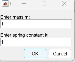
We get a default input dialogue box with value of m and k as 1 after we run the script file.

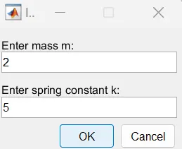
We set the value of m=2and k=5 for our reference and run the program.

We get the ode45 and ode23 plots for the system as follows:

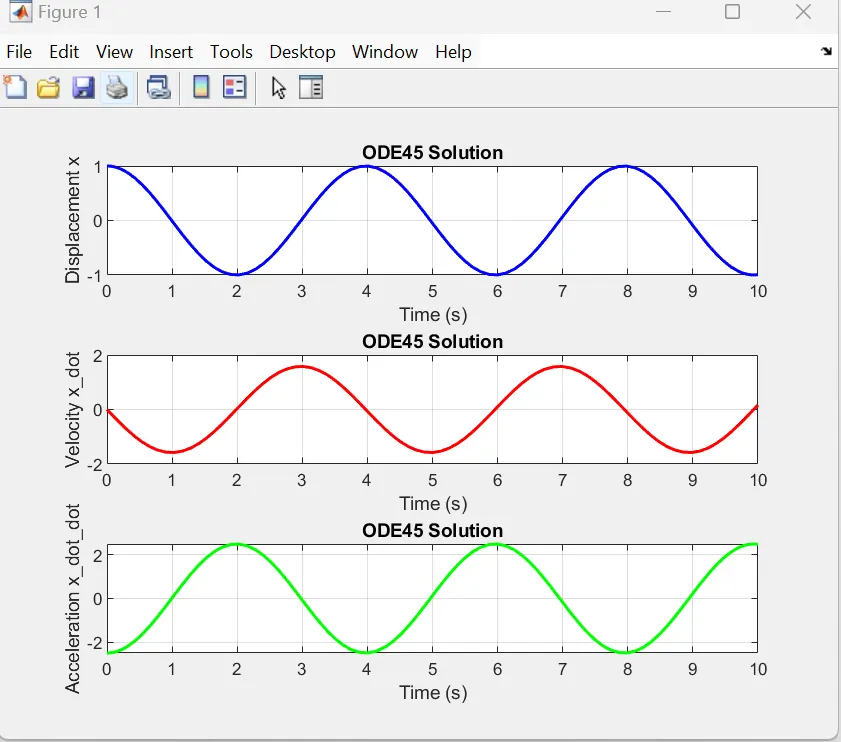
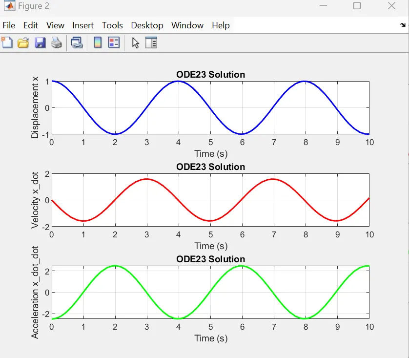
Observation: ode45 plot results are likely to provide smoother and more accurate solutions than ode 23 plots but in this case of simple harmonic oscillator the plot results and contours are almost similar.

Project 2:

MATLAB CODE:

% Load the data from International standard atmosphere tables file

data = readmatrix('ISA_PROJECT1_Q2_DATA.xlsx');

altitudes = data(:, 1); % Since first column is altitude

temperatures = data(:, 2); % Since second column is temperature

% Polynomial degree (e.g., 2 for quadratic)

degree = 2;

% Fit a polynomial model

coefficients = polyfit(altitudes, temperatures, degree);

% Evaluate the polynomial model

evaluated_temperatures = polyval(coefficients, altitudes);

% Determine goodness of fit

SStot = sum((temperatures - mean(temperatures)).^2);%Total Sum of Squares

SSres = sum((temperatures - evaluated_temperatures).^2);%Sum of Squares of Residuals

R2 = 1 - (SSres / SStot);%R-squared value

% Display goodness of fit

fprintf('Goodness of Fit (R-squared): %.4f\n', R2);

% Generate comparative plot

figure;

plot(altitudes, temperatures, 'o', 'DisplayName', 'Original Data');

hold on;

plot(altitudes, evaluated_temperatures, '-', 'DisplayName', 'Polynomial Fit');

xlabel('Altitude (m)');

ylabel('Temperature (°C)');

title('Altitude vs Temperature');

legend('show');

grid on;

hold off;

% Create a table for better formatting with row names

T = table(altitudes, evaluated_temperatures, 'VariableNames', {'Altitude', 'EvaluatedTemperature'});

% Write the table to a text file

writetable(T, 'evaluated_data.txt', 'Delimiter', 'tab');

disp('Evaluated data saved to evaluated_data.txt');

Explanation:

The code line data = readmatrix('ISA_PROJECT1_Q2_DATA.xlsx'); reads data from an Excel file named ISA_PROJECT1_Q2_DATA.xlsx.

It assumes that the file contains two columns: the first column for altitude and the second for temperature.

degree=2 code line specifies that a quadratic polynomial (degree 2) will be used to fit the data.

polyfit-Fits a polynomial of the specified degree to the data and returns the polynomial coefficients.

SStot calculates the total variability in the observed temperatures. It represents how much the observed values deviate from their mean value.

SSres calculates the variability not explained by the polynomial model. It quantifies how much the predicted values (from the polynomial model) deviate from the actual observed values.

R2 computes the R-squared value, indicating the proportion of variance explained by the model. The R-squared value is derived from SStot and SSres and provides a measure of how well the polynomial model explains the variability in the data.

An R-squared value close to 1 indicates a good fit, meaning most of the variability in the data is explained by the model.

An R-squared value close to 0 indicates a poor fit, meaning the model does not explain much of the variability in the data.

Code-T = table(altitudes, evaluated_temperatures, 'VariableNames', {'Altitude', 'EvaluatedTemperature'}) , creates a table with columns for altitudes and the evaluated temperatures.

Code line : writetable(T, 'evaluated_data.txt', 'Delimiter', 'tab'), saves this table to a text file named evaluated_data.txt with tab delimiters.

Output:

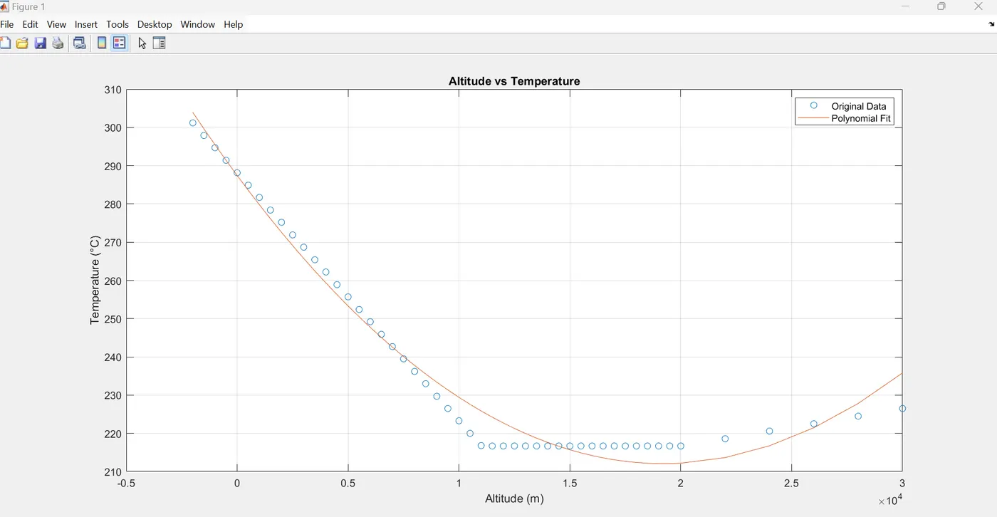
Observation: The R-squared value for the given set of data is 0.9811. Hence as discussed , an R-squared value close to 1 indicates a good fit, meaning most of the variability in the data is explained by the model.

Project 3:

MATLAB CODE:

function y = myFunction(x)

y = sin(x.^2) + cos(x) - 2*sin(x).*cos(x);

end

x = linspace(-2*pi, 2*pi, 1000);

y = myFunction(x);

figure;

plot(x, y);

xlabel('x');

ylabel('y');

title('Plot of y = sin(x^2) + cos(x) - 2 sin(x) cos(x)');

grid on;

% Define the function for minimization

function y = objectiveFunction(x)

y = myFunction(x);

end

% Initial guess for fminsearch

initialGuess = [-2*pi; 2*pi];

% Find local minima

localMinima = [];

for i = 1:length(initialGuess)

[xMin, yMin] = fminsearch(@objectiveFunction, initialGuess(i));

localMinima = [localMinima; xMin, objectiveFunction(xMin)];

end

% Find global maximum

[xMax, yMax] = fminsearch(@(x) -objectiveFunction(x), 0);

yMax = -objectiveFunction(xMax);

globalMaxima = [xMax, yMax];

% Collect all points

extrema = [localMinima; globalMaxima];

figure;

plot(x, y, 'b-', 'LineWidth', 2);

hold on;

plot(localMinima(:,1), localMinima(:,2), 'ro', 'MarkerFaceColor', 'r');

plot(globalMaxima(1), globalMaxima(2), 'go', 'MarkerFaceColor', 'g');

% Highlight local minima

for i = 1:size(localMinima, 1)

text(localMinima(i,1), localMinima(i,2), sprintf('Min (%.2f, %.2f)', localMinima(i,1), localMinima(i,2)), 'VerticalAlignment', 'bottom', 'HorizontalAlignment', 'right');

end

% Highlight global maximum

text(globalMaxima(1), globalMaxima(2), sprintf('Max (%.2f, %.2f)', globalMaxima(1), globalMaxima(2)), 'VerticalAlignment', 'bottom', 'HorizontalAlignment', 'left');

xlabel('x');

ylabel('y');

title('Plot of y = sin(x^2) + cos(x) - 2 sin(x) cos(x) with Local Minima and Global Maxima');

grid on;

legend('Function', 'Local Minima', 'Global Maximum');

% Use gtext to allow manual placement of text if needed

gtext('Local Minima');

gtext('Global Maxima');

hold off;

Explanation:

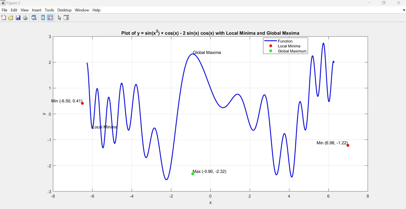
initialGuess provides starting points for fminsearch to find local minima.

We initialize an empty array localMinima to store the local minima.

The program iterates through each initial guess, uses fminsearch to find the minimum value starting from that guess, and stores the results in localMinima.

To find the global maximum, fminsearch is used to minimize the negative of objectiveFunction, effectively finding the maximum of the original function.

Sets an initial guess of 0 for the global maximum search.

After finding xMax, yMax is computed by negating the result of objectiveFunction at xMax and stores the result in globalMaxima.

By using gtext, we can position text more precisely according to our preferences on the plot.

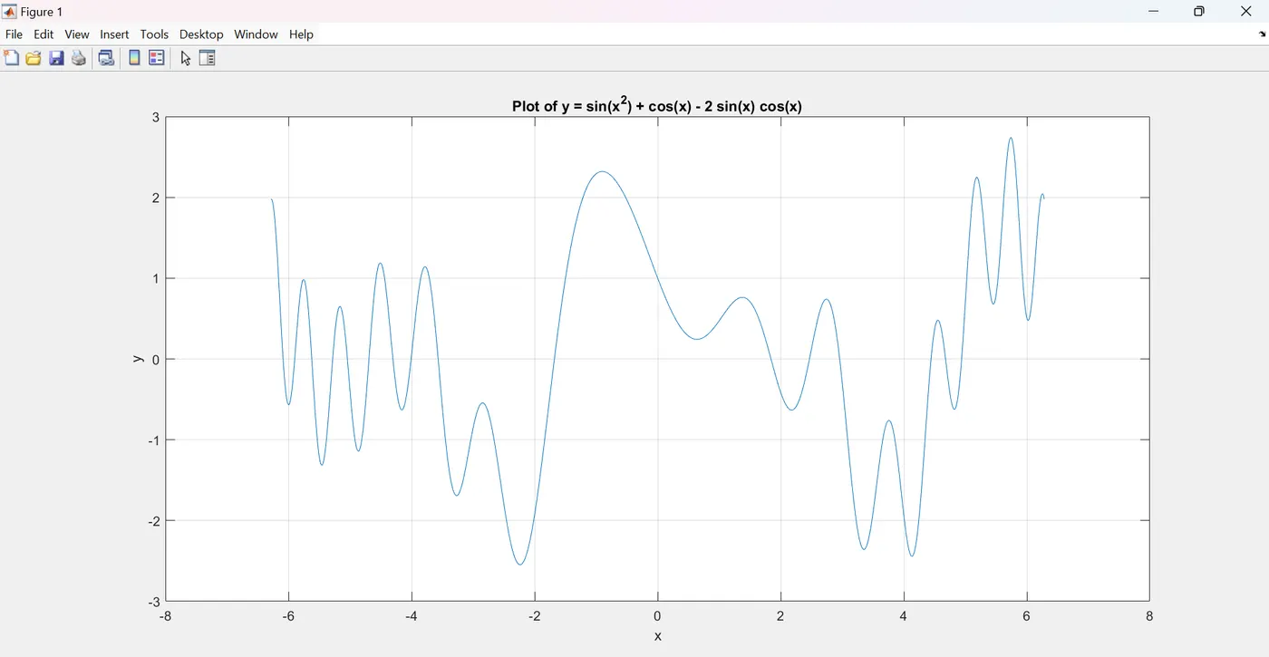
OUTPUT:

Project 4:

MATLAB CODE

%Reference example for contour command

% Define the grid of points

[x, y] = meshgrid(-3:0.1:3, -3:0.1:3);

% Define the function to plot

z = sin(sqrt(x.^2 + y.^2)); % Calculate Z values

% Create a contour plot

figure;

contour(x, y, z, 20); % 20 contour levels

colorbar; % Show color scale

xlabel('x');

ylabel('y');

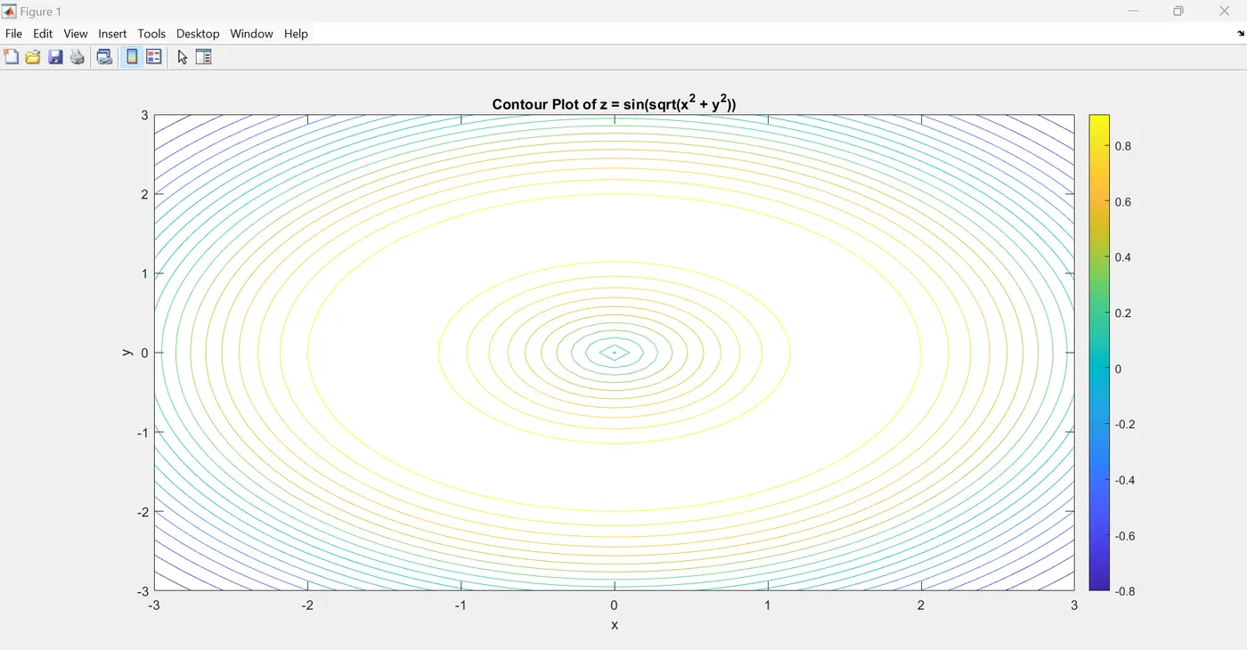
title('Contour Plot of z = sin(sqrt(x^2 + y^2))');

[x, y] = meshgrid(-3:0.1:3, -3:0.1:3);

Explanation:

meshgrid creates a grid of points over the specified ranges. In this case, it creates a grid where both x and y range from -3 to 3 with a step size of 0.1.

x and y are matrices where each element represents coordinates of points in the grid. For example, x contains repeated rows of x-coordinates and y contains repeated columns of y-coordinates.

z is computed as sin(sqrt(x.^2 + y.^2)). This calculates the value of z at each grid point based on the distance from the origin (0,0).

sqrt(x.^2 + y.^2) computes the Euclidean distance from the origin, and sin applies the sine function to this distance. This results in a function that depends only on the radial distance from the origin, creating concentric wave patterns.

figure; opens a new figure window.

contour(x, y, z, 20)- creates a ‘contour plot’ of the function z.

· x and y provide the coordinates for the grid points.

· z provides the function values at those coordinates.

· 20 specifies the number of contour levels to the plot. MATLAB will automatically determine contour levels between the minimum and maximum values of z, and plot lines where the function z has constant values.

colorbar adds a color scale bar to the plot, which indicates the mapping of contour levels to colors.

xlabel('x'); labels the x-axis as 'x'.

ylabel('y'); labels the y-axis as 'y'.

title('Contour Plot of z = sin(sqrt(x^2 + y^2))'); adds a title to the plot describing the function that was plotted.