Project 1

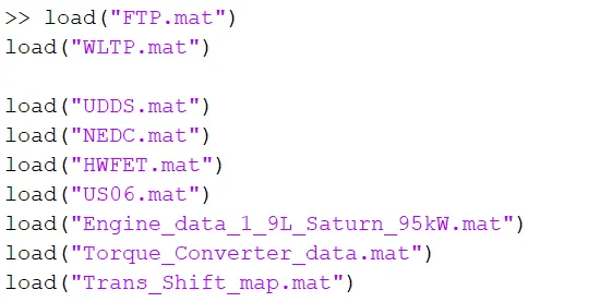
We load the required drive cycle, engine parameters files in the command window as follows:

“Project1_InitFile.m” MATLAB script:

% Initialization file for loading the variables for the Conventional vehicle simulation model

%% Vehicle Parameters

M = 1500; % Vehicle weight [kg]

Cr = 0.015; % Rolling resistance coefficient

Rw = 0.35; % Rolling radius [m]

Cd = 0.33; % Drag coefficient

Af = 2; % Frontal area [m2]

rhoa = 1.225; % Air density [kg/m3]

Vwind = 0; % Wind velocity [kmph]

g = 9.81; % Gravitational acceleration [m/s2]

theta = 0; % Slope [deg]

myu_road_tire = 1; % Coefficient of friction between tire - road interface

%% Powertrain Parameters

FDR = 3.73; % Final Drive Ratio / Diff Ratio

DiffEff = 0.99; % Differential efficiency (assumed independent of operating conditions)

NumGear = 4; % Number of gears in transmission

TransGear = [1:NumGear]; % Transmission Gears

TransRatio = [3.06, 1.62, 1, 0.7]; % Corresponding Transmission ratios

TransEff = 0.90; % Transmission efficiency (assumed independent of operating conditions)

TC_SR = [0, .5, .6, .7, .8, .87, .92, .94, .96, .97, 1]; % Torque Converter Speed Ratio (Matlab default) -> TurbSpd/PumpSpd

TC_TR = [2.232, 1.5462, 1.4058, 1.2746, 1.1528, 1.0732, 1.0192, 1, 1, 1, 1]; % Torque Converter Torque Ratio (Matlab default) -> TurbTrq/PumpTrq

TC_Cf = 1e-4 * [.72558, .66322, .63463, .59042, .51331, .4144, .29287, .22444, .12186, .04386, 0]; % Torque Converter Capacity Factor (Matlab default) -> PumpTrq/PumpSpd^2 [Nm/rpm^2]

load Engine_data_1_9L_Saturn_95kW

load Trans_Shift_map

%% Driver Parameters

Kp = 10; % P gain for driver PI model

Ki = 1; % I gain for driver PI model

Drive_Cycle_Select = 2; % Drive cycle selection

% Drive cycle values in m/s

if Drive_Cycle_Select == 1

load DriveCycles/UDDS;

elseif Drive_Cycle_Select == 2

load HWFET;

elseif Drive_Cycle_Select == 3

load DriveCycles/FTP;

elseif Drive_Cycle_Select == 4

load DriveCycles/US06;

elseif Drive_Cycle_Select == 5

load DriveCycles/NEDC;

elseif Drive_Cycle_Select == 6

load DriveCycles/WLTP;

end

time_end = cyc_time(end);

vel_end = cyc_vel(end);

Vehicle Parameters

This section defines the basic parameters related to the vehicle's physical characteristics and performance attributes.

• M: Vehicle weight in kilograms (1500 kg is typical for a mid-size car).
• Cr: Rolling resistance coefficient, which influences how much energy is lost to friction as the vehicle rolls.
• Rw: Rolling radius in meters, related to how far the vehicle travels with each wheel rotation.
• Cd: Drag coefficient, affecting aerodynamic drag; lower values indicate better aerodynamics.
• Af: Frontal area in square meters, another factor in aerodynamic drag calculations.
• rhoa: Air density in kg/m³, used in drag force calculations.
• Vwind: Wind velocity in km/h; currently set to 0, implying no wind resistance.
• g: Gravitational acceleration in m/s², used for calculating forces on inclines.
• theta: Road slope in degrees; here, it is set to 0 (flat terrain).
• myu_road_tire: Coefficient of friction between tires and the road, which affects traction.

2. Powertrain Parameters

This section specifies the powertrain characteristics, which are crucial for simulating how the vehicle accelerates and handles.

• FDR: Final Drive Ratio, determining how engine RPM translates to wheel RPM.
• DiffEff: Differential efficiency, assumed to be constant; represents losses in the differential.
• NumGear: Number of gears in the transmission; here, it's set to 4.
• TransGear: Array representing each gear in the transmission (1 to NumGear).
• TransRatio: Specific gear ratios for each transmission gear, affecting acceleration and top speed.
• TransEff: Transmission efficiency, indicating how much of the engine's power is transmitted to the wheels.

Torque Converter Parameters

• TC_SR: Torque converter speed ratios, indicating how turbine speed relates to pump speed.
• TC_TR: Torque converter torque ratios, showing the relationship between turbine torque and pump torque.
• TC_Cf: Torque converter capacity factors, used for calculating pump torque based on pump speed.

3. Loading Engine and Transmission Data

• load Engine_data_1_9L_Saturn_95kW: This command loads pre-defined engine characteristics (likely from a .mat file) for a specific engine model.
• load Trans_Shift_map: Loads a shift map for the transmission, which is essential for simulating gear changes.

4. Driver Parameters

This section sets parameters for the driver model, simulating how a driver reacts to speed changes.

• Kp and Ki: These are gains for a Proportional-Integral (PI) controller, which helps the driver model adjust throttle based on speed feedback.
• Drive_Cycle_Select: An integer that selects which drive cycle to simulate.

5. Drive Cycle Loading

Depending on the value of Drive_Cycle_Select, the script loads different driving patterns:

• if statements: These conditionally load drive cycle data (e.g., UDDS, HWFET, etc.) based on the selected index. Each of these cycles represents different driving conditions, such as urban or highway driving.

6. End of Simulation Parameters

• time_end: Captures the end time of the selected drive cycle from the cyc_time variable.
• vel_end: Captures the end velocity of the drive cycle from the cyc_vel variable.

This initialization file sets up all necessary parameters and data to simulate a conventional vehicle's dynamics under various driving conditions. By adjusting these parameters, we can study how the vehicle behaves under different scenarios, which is crucial for design and analysis in automotive engineering.

“Project1_ProcessingFile.m”

%% Post-Processing File

% File for post-processing the Conventional vehicle simulation model data

Time = out.tout;

Acc_Pdl = out.Acc_Pdl; % Accelerator pedal [%]

Brk_Pdl = out.Brk_Pdl; % Brake pedal [%]

Gear_Cmd = out.Gear_Cmd; % Transmission gear

Trans_In_Spd = out.Trans_In_Spd*30/pi; % Transmission input speed [rpm]

Trans_Out_Spd = out.Trans_Out_Spd*30/pi;% Transmission output speed [rpm]

Eng_Trq = out.Eng_Trq; % Engine brake torque [Nm]

Eng_Spd = out.Eng_Spd*30/pi; % Engine speed [rpm]

Eng_Fuel_rate = out.Eng_Fuel_Rate; % Engine Fuel Rate [g\kW]

Eng_Fuel_Consump = out.Eng_Fuel_Consumption; % Engine fuel consumption [g]

Veh_Dist = out.Veh_Dist/1000; % Distance traveled by vehicle [km]

Veh_Spd = out.Veh_Spd*18/5; % Vehicle speed [kmph]

Whl_Spd = out.Whl_spd*30/pi; % Wheel speed [rpm]

Desired_spd = out.Desired_Velo*18/5; % Desired Speed [Kmph]

%% Data Analysis

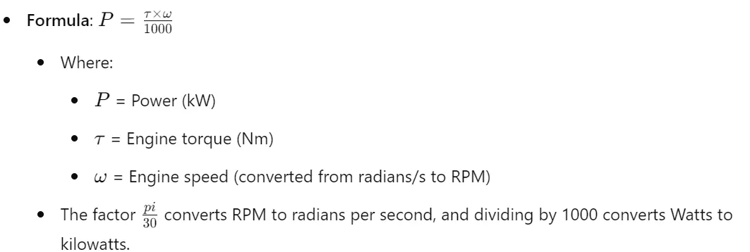
Eng_Pwr = Eng_Spd*pi/30.*Eng_Trq/1000; % Engine brake power [kW]

rho_petrol = 0.7197; % Density of petrol [kg/L]

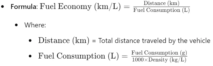
kmpl = Veh_Dist(end)/(Eng_Fuel_Consump(end)/1000/rho_petrol); % Fuel economy [kmpl]

% Display Fuel Economy of the Cycle

fprintf('\nFuel Economy = %2.2fKmpl\n\n',kmpl);

%% Plotting vehicle characteristics time trace

% Plotting transmission input, transmission output and wheel speed

% Figure 1 Legend

legend({'Trans Input', 'Trans Output', 'Wheel Speed', ...

sprintf('Time: %.1f to %.1f s', Time(1), Time(end))});

% Figure 2 Subplot 1 Legend

legend({sprintf('Torque: %.1f to %.1f Nm', min(Eng_Trq), max(Eng_Trq)), ...

sprintf('Time: %.1f to %.1f s', Time(1), Time(end))});

% Figure 2 Subplot 2 Legend

legend({sprintf('Power: %.1f to %.1f kW', min(Eng_Pwr), max(Eng_Pwr)), ...

sprintf('Time: %.1f to %.1f s', Time(1), Time(end))});

% Figure 2 Subplot 3 Legend

legend({sprintf('Fuel Rate: %.1f to %.1f g/kW', min(Eng_Fuel_rate), max(Eng_Fuel_rate)), ...

sprintf('Time: %.1f to %.1f s', Time(1), Time(end))});

% Figure 2 Subplot 4 Legend

legend({sprintf('Fuel Consumption: %.1f to %.1f g', min(Eng_Fuel_Consump), max(Eng_Fuel_Consump)), ...

sprintf('Time: %.1f to %.1f s', Time(1), Time(end))});

% Figure 3 Subplot 1 Legend

legend({'Accel', 'Brake', ...

sprintf('Time: %.1f to %.1f s', Time(1), Time(end))});

% Figure 3 Subplot 2 Legend

legend({sprintf('Gear Command: %.1f to %.1f', min(Gear_Cmd), max(Gear_Cmd)), ...

sprintf('Time: %.1f to %.1f s', Time(1), Time(end))});

% Figure 3 Subplot 3 Legend

legend({'Actual speed', 'Desired speed', ...

sprintf('Time: %.1f to %.1f s', Time(1), Time(end))});

% Figure 3 Subplot 4 Legend

legend({sprintf('Distance: %.1f to %.1f km', min(Veh_Dist), max(Veh_Dist)), ...

sprintf('Time: %.1f to %.1f s', Time(1), Time(end))});

% Figure 4 Legend

legend({sprintf('Drive Cycle Time: %.1f to %.1f s', cyc_time(1), cyc_time(end))});

% Engine Operating Points Legend

legend({'Max Curve', 'Operating Points', ...

sprintf('Time: %.1f to %.1f s', Time(1), Time(end))});

%% Plotting Drive Cycle

figure(4)

hold on

grid on

plot(cyc_time, cyc_vel, 'linewidth', 1, 'Color', 'black');

xlabel('Time [s]')

ylabel('Velocity [Mph]')

title('Drive Cycle')

% Test Results

Avg_speed = sum(Veh_Spd)/length(Veh_Spd);

Max_Speed = maxk(Veh_Spd,1);

table(Avg_speed,Max_Speed,kmpl,'VariableNames',{'Average Speed [kmph]','Maximum Speed [kmph]','Fuel Economy [kmpl]'})

%% Plotting engine operating points on engine fuel map

figure('Name','Engine Operating Points');

hold on

grid on

title('Engine Operating Points','fontsize',12);

p1=plot(Eng_map_spd*30/pi,Eng_max_trq,'linewidth',2,'color','r');

p2=line([Eng_map_spd(end)*30/pi Eng_map_spd(end)*30/pi],[0 Eng_max_trq(end)]);

set(p2,'linewidth',1,'linestyle','--','color','k');

p3=line([Eng_map_spd(1)*30/pi Eng_map_spd(1)*30/pi],[0 Eng_max_trq(1)]);

set(p3,'linewidth',1,'linestyle','--','color','k');

[c,h] = contour(Eng_map_spd'*30/pi,Eng_map_trq,Eng_fuel_map');

clabel(c,h);

xlabel('Engine Speed [rpm]');

ylabel('Engine Torque [Nm]');

title('Engine Fuel Consumption Map [g/s]');

legend({'Max Curve','Operating Points'});

axis([Eng_map_spd(1)*30/pi Eng_map_spd(end)*30/pi 0 Eng_map_trq(end)]);

The post-processing file is used for analyzing the data from the conventional vehicle simulation model. The following working formulae are involved in the analysis :

Engine Brake Power Calculation:

Fuel Economy Calculation:

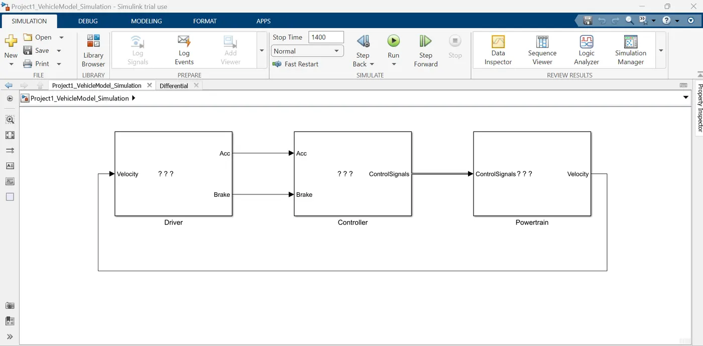
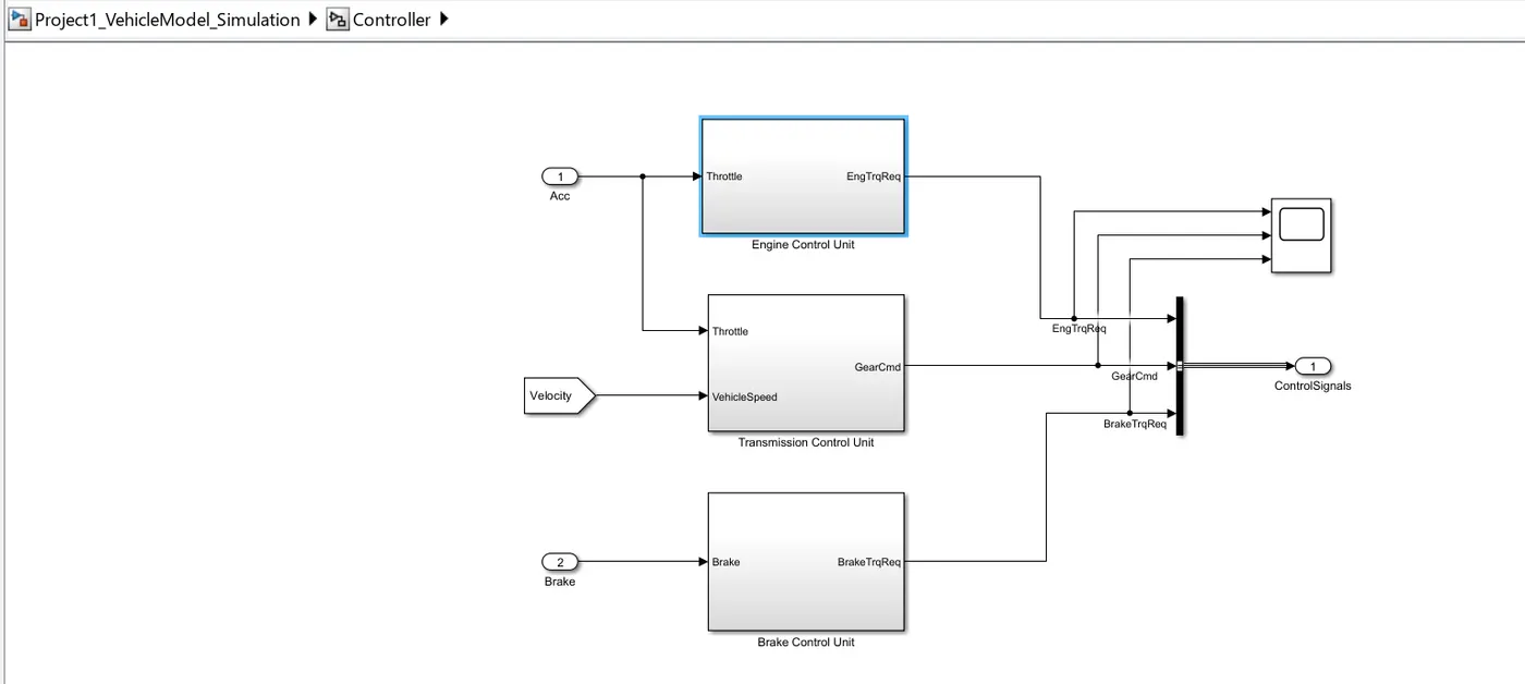
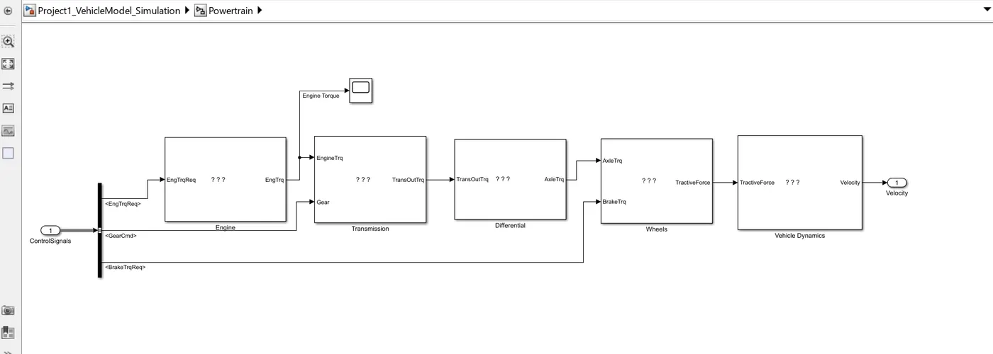
The Simulink model "Project1_VehicleModel_Simulation.slx" simulates a vehicle featuring a 'Driver' block that functions as a basic PI controller. This block generates accelerator and brake pedal outputs to align the desired and actual vehicle speeds. The 'Controller' block serves as the vehicle's electronic control unit, processing the driver inputs to produce the desired engine torque, transmission gear, and brake torque. These outputs are then directed to the 'Powertrain' block, which models the drivetrain, including an 'Engine' linked to an 'Automatic Transmission' via a 'Torque Converter.' The transmission's output connects to the 'Differential,' which drives the 'Wheels' and generates the tractive force needed for vehicle acceleration. The 'Vehicle Dynamics' block captures the longitudinal dynamics of the vehicle, including road load effects. The simulation uses a fixed step size of 0.01 seconds with the ode3 solver.

The Vehicle SIMULINK model consists of three subsystems: Driver, Controller, Powertrain

The DRIVER subsystem contains the following SIMULINK blocks:

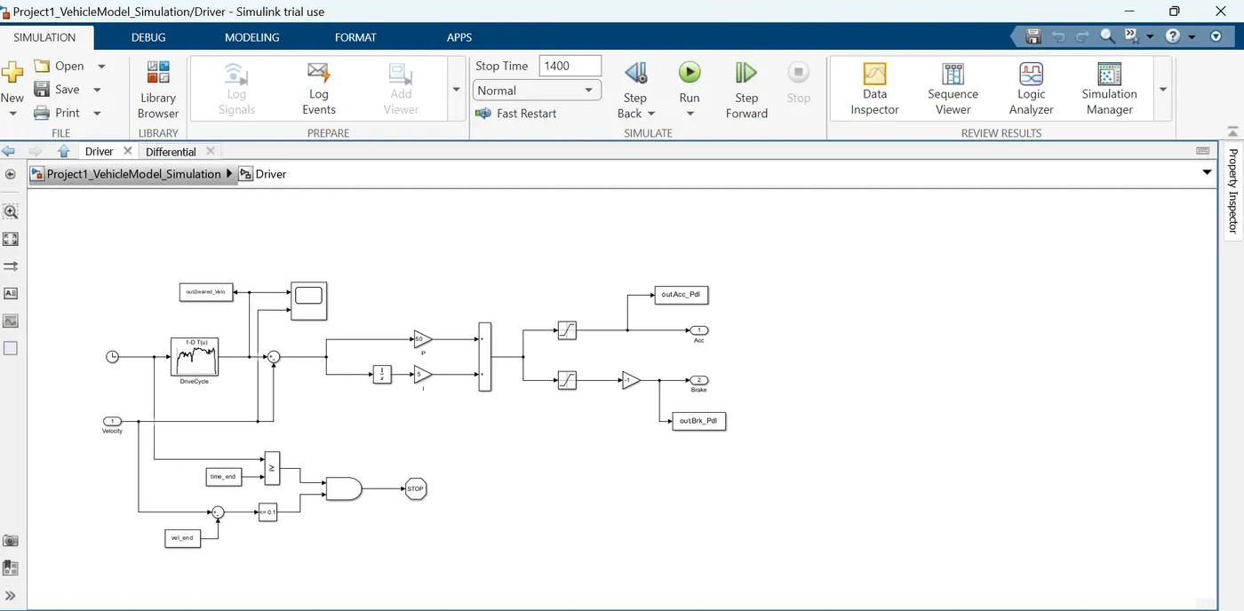
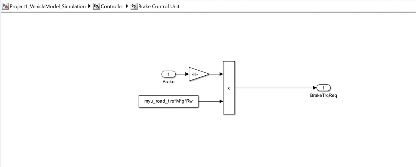
The Controller subsystem consists of following subsystems-Engine Control Unit, Transmission Control Unit, Brake Control Unit:

The Engine torque, gear CMD and Brake torque characteristics plot (from SCOPE block)are as follows:

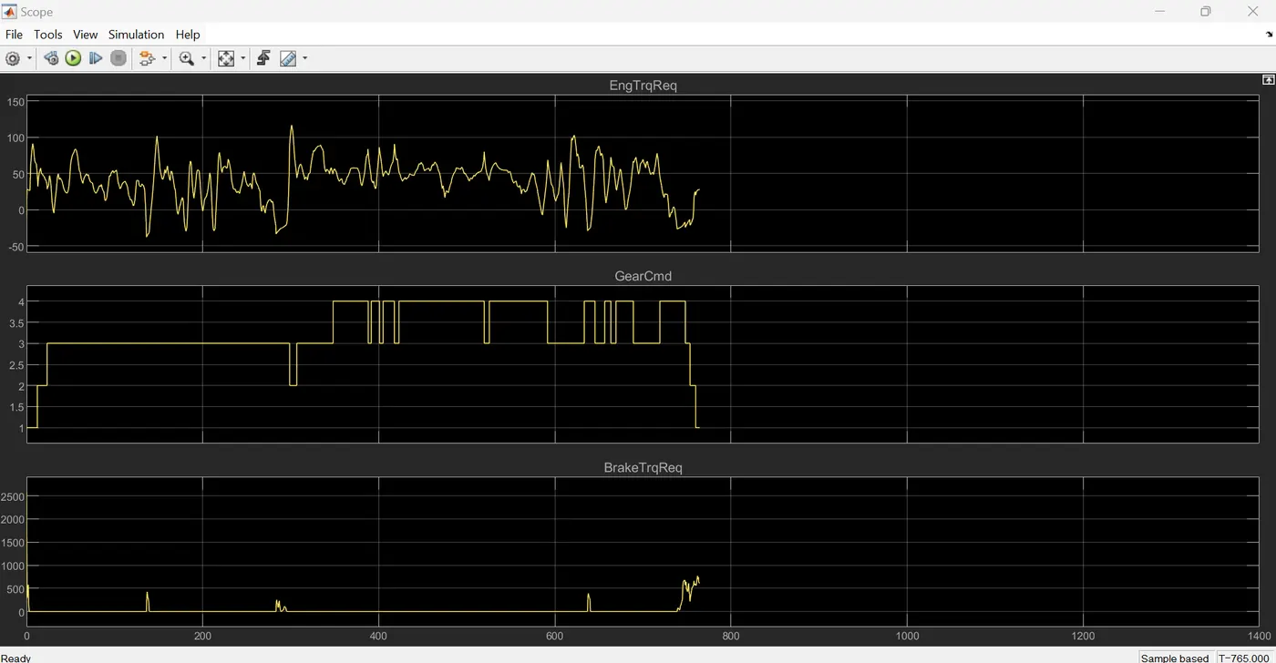
EngTrqReq -The line shows variations in the torque demand, due to changes in load or operating conditions.

GearCmd-Plot represents step function representing the gear changes. Each step indicates a shift to a new gear level. The plot shows the sequence of gear changes over time.

BrakeTrqReq-Plot represents a series of spikes representing braking events. The height of each spike indicates the magnitude of the braking force applied with respect to time. The plot shows the timing and intensity of braking actions.

Now, The Engine Control Unit has following blocks:

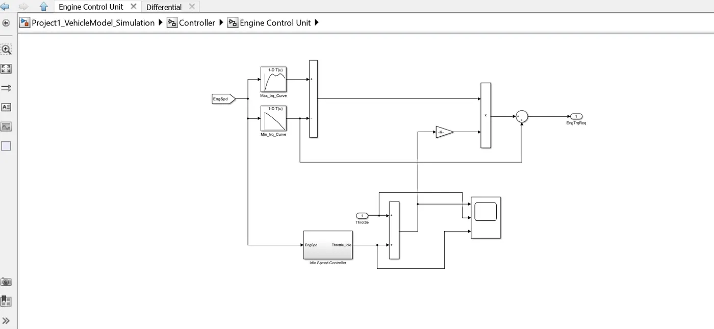
Throttle and idle speed controller plots from scope block is mentioned below:

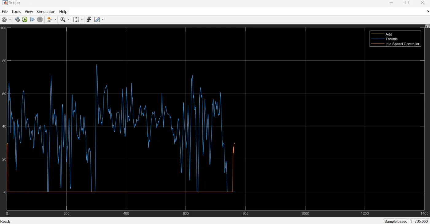
The plot illustrates how the throttle and idle speed controller interact over time. The given relationship between the two plot lines suggests a correlation between throttle position and idle speed. When the throttle is opened (blue line increases), the idle speed controller may adjust the engine speed (orange line) to maintain a desired idle RPM or prevent excessive engine speed.

The' Idle speed controller subsystem' of Engine Control Unit has following blocks:

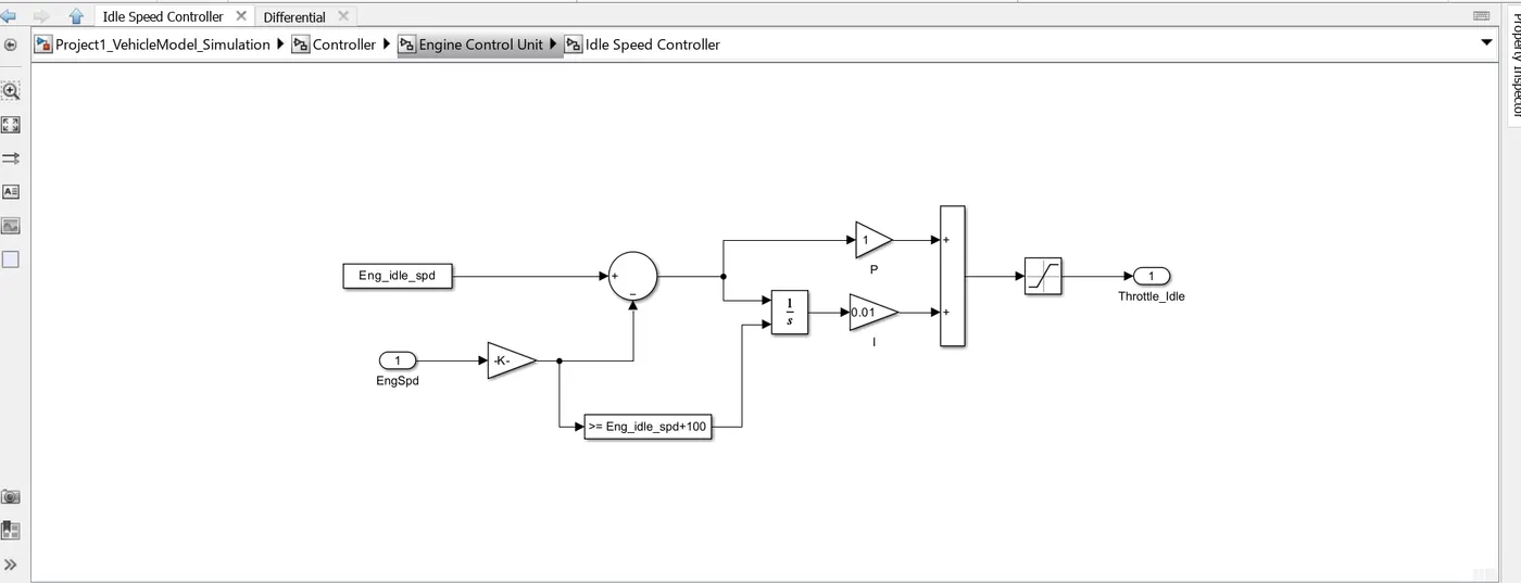
The ' Transmission Control Unit subsystem' of Engine Control Unit has following blocks:

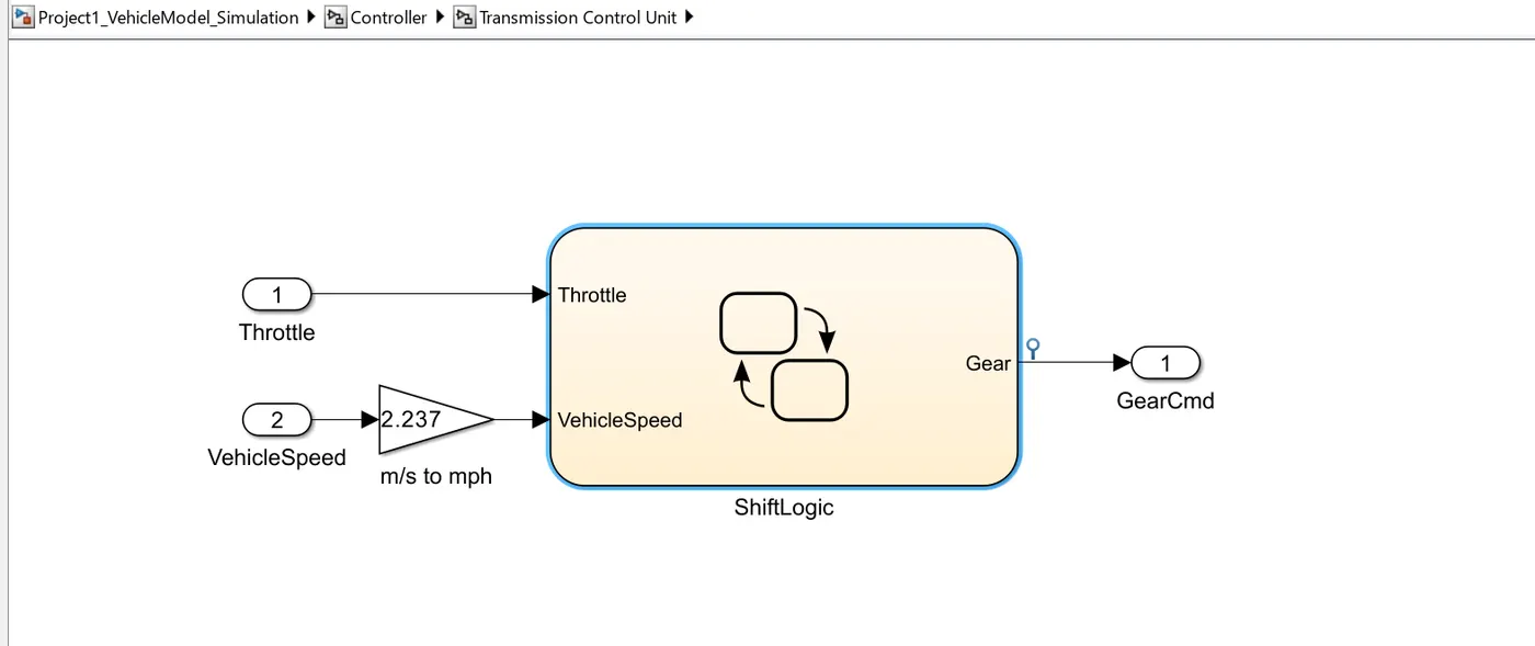The subsystem has following state flow:

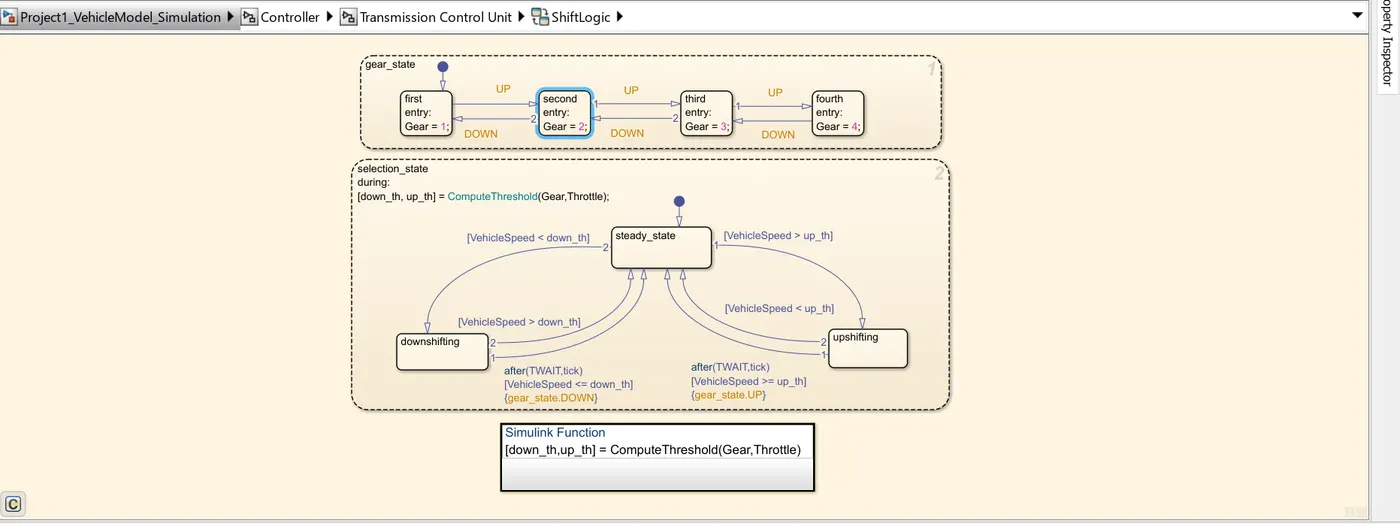
The' controller subsystem' of Engine Control Unit has following blocks:

The Powertrain subsystem has following blocks:

The plot from the scope block of above system is as follows:

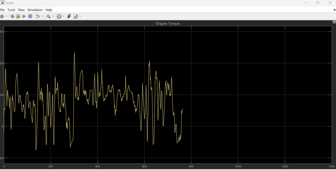
Above plot illustrates the variation of engine torque over time. The line shows fluctuations in the torque output, due to changes in load, operating conditions, or control inputs.

The Engine subsystem of powertrain system is as follows:

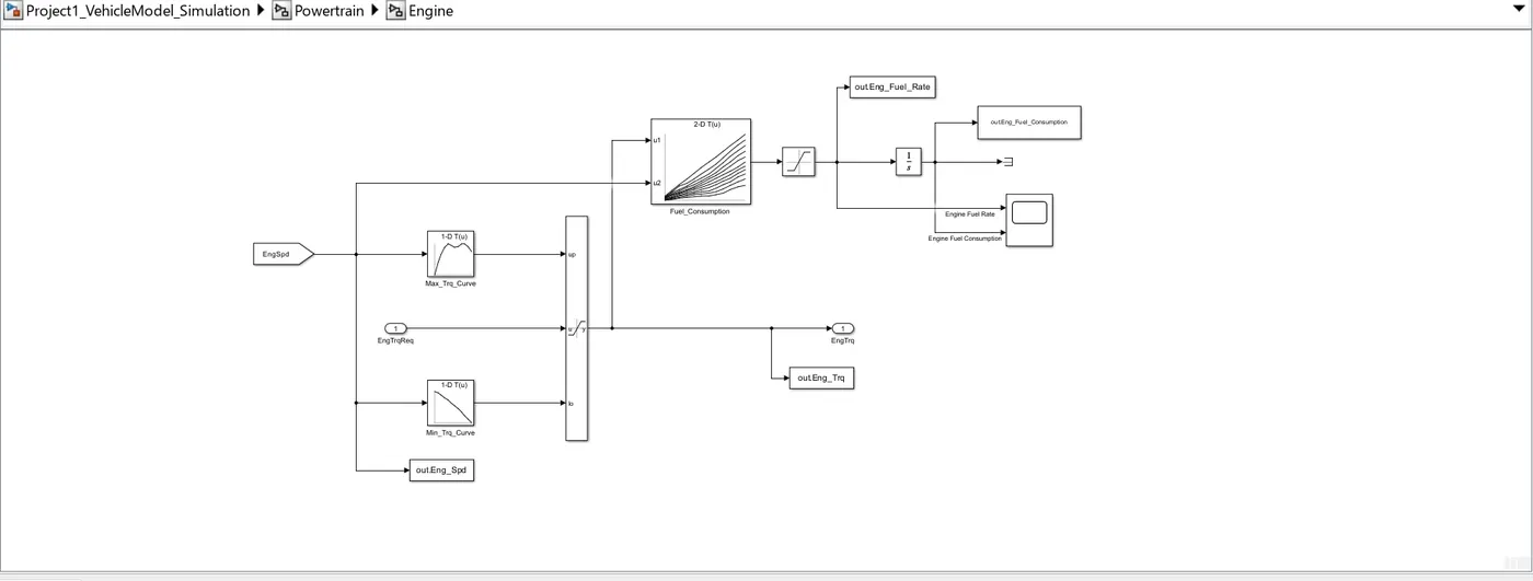
The plot from the scope block of above system is as follows:

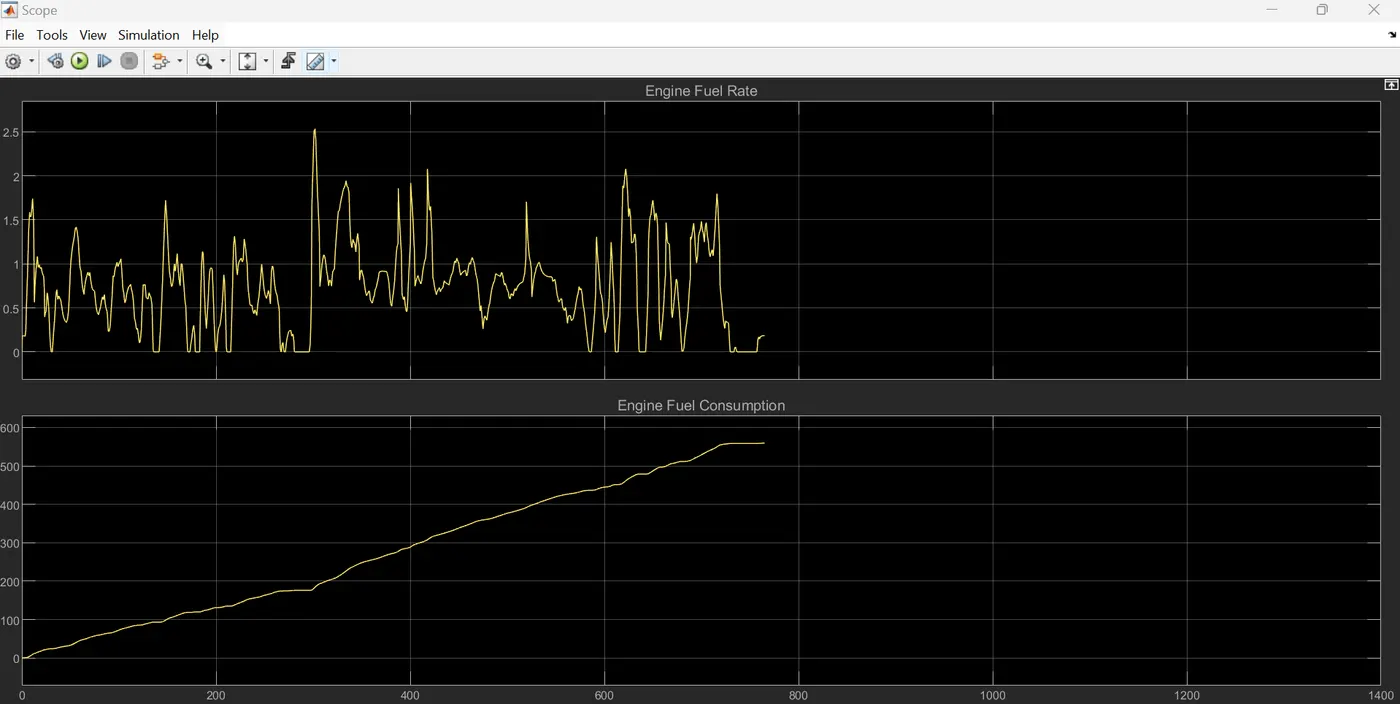
A fluctuating line representing the instantaneous engine fuel consumption rate over time. The line shows variations in fuel consumption due to changes in load, speed, or operating conditions.

An increasing line representing the cumulative engine fuel consumption over time. The line shows the total amount of fuel consumed as the engine operates.

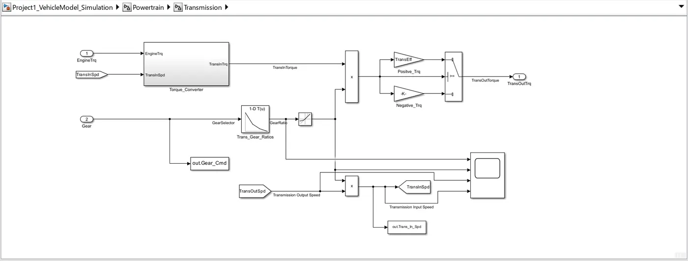
The Transmission subsystem of powertrain system is as follows:

The plot from the scope block of above system is as follows:

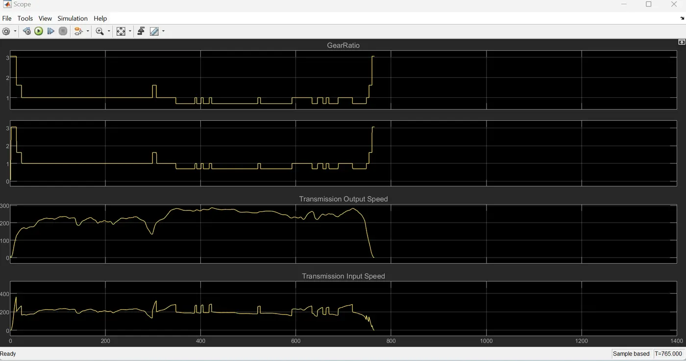
Observations from above plots:

GearRatio: A step function representing the gear changes. Each step indicates a shift to a new gear ratio. The plot shows the sequence of gear changes over time.

Transmission Output Speed: fluctuating line representing the rotational speed of the transmission's output shaft over time. The line shows variations in output speed, due to changes in engine torque, gear shifts, or load conditions.

Transmission Input Speed: A fluctuating line representing the rotational speed of the transmission's input shaft over time. The line shows variations in input speed, likely driven by the engine's rotational speed.

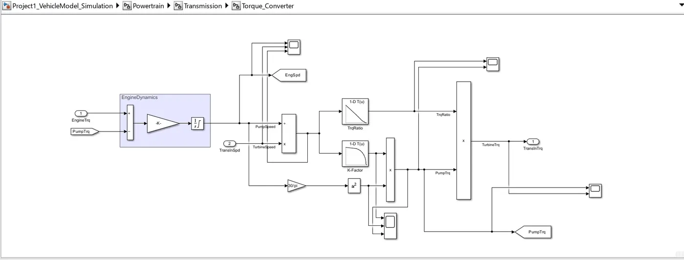
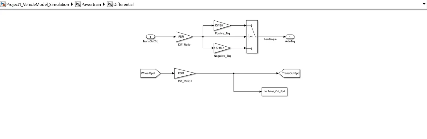
The Differential subsystem of powertrain system is as follows:

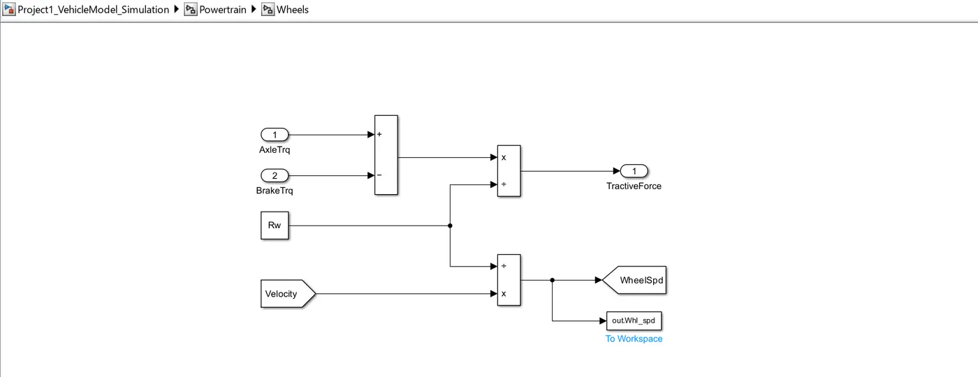
The Wheel subsystem of powertrain system is as follows:

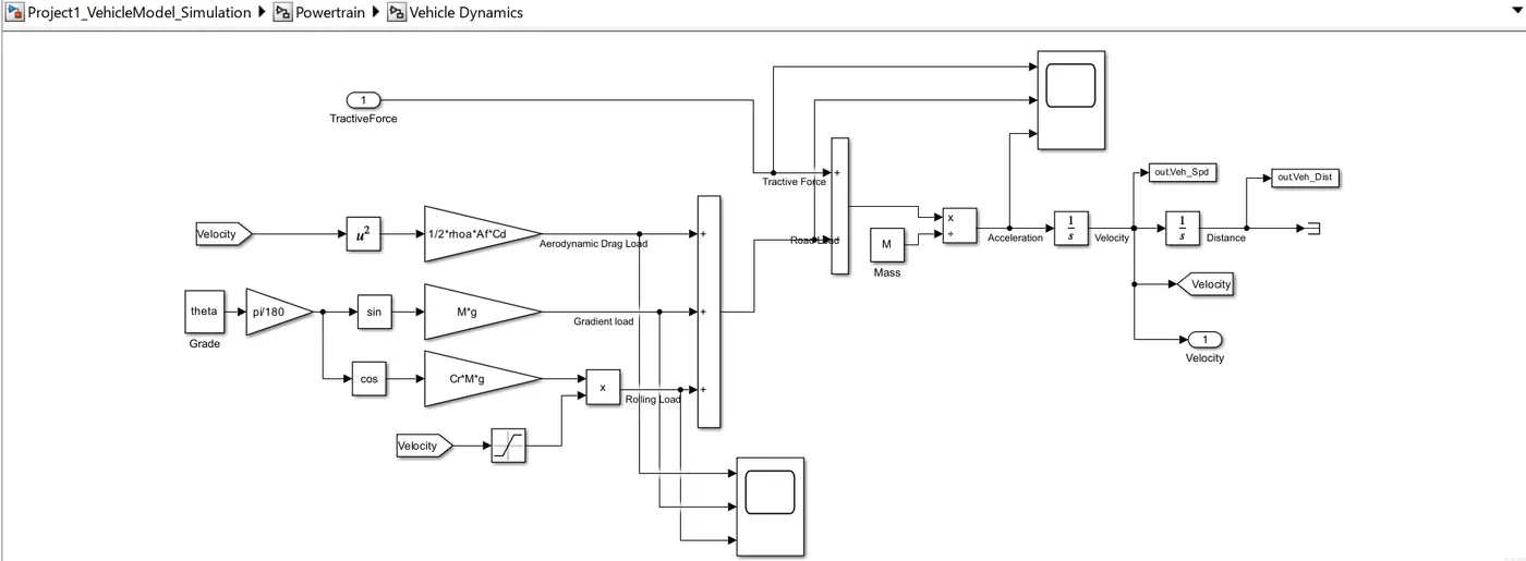
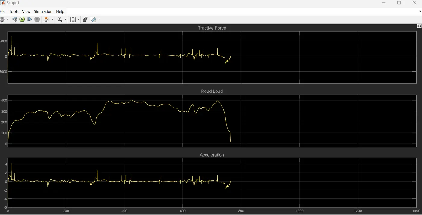
The plot from the scope blocks of above sub-system is as follows:

Observations from above plots:

• The tractive force fluctuates over time, likely due to changes in engine power, gear selection, and road conditions.
• The road load also varies, primarily influenced by changes in speed and road surface.
• The acceleration is directly related to the difference between tractive force and road load. When tractive force exceeds road load, the vehicle accelerates; when road load exceeds tractive force, the vehicle decelerates.

The specific values and trends in the plots may vary depending on the vehicle, driving conditions, and the purpose of the simulation.

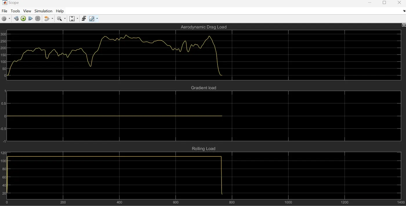
Observations from above plots:

• Aerodynamic Drag Load: A fluctuating line representing the aerodynamic drag force acting on the system over time. The line shows variations in drag due to changes in speed or other factors affecting air resistance.
• Gradient Load: A flat line at zero, indicating that there is no gradient load acting on the system throughout the time period. This could suggest that the system is operating on flat terrain or that the gradient load is negligible compared to other forces.

• Rolling Load: A step function with two levels, indicating a change in rolling load at a specific time. The plot suggests that there is a sudden increase in rolling load, followed by a constant level. This could be due to changes in road conditions, such as transitioning from a flat surface to an incline.

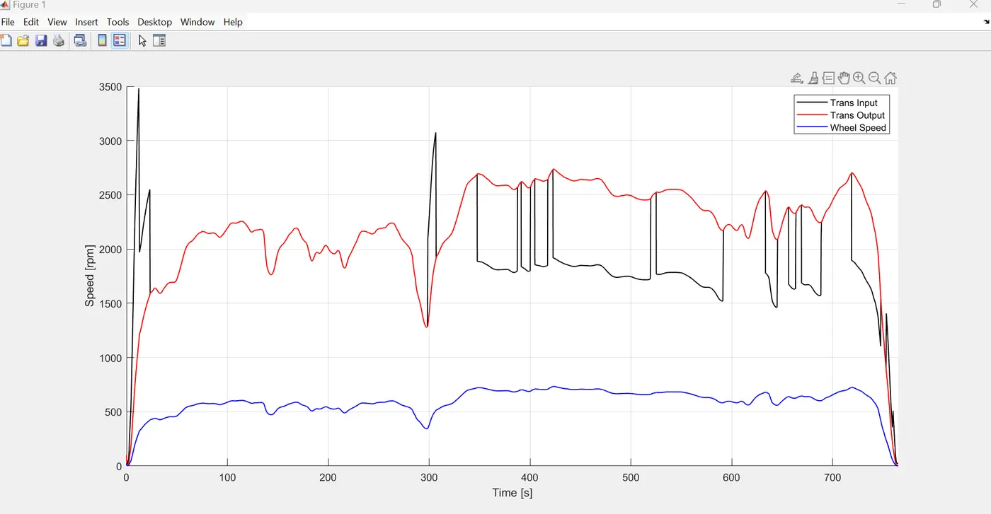
The plot illustrates how the rotational speed of the engine (transmission input) is transformed through the transmission to the wheels. The relationship between these speeds is influenced by the gear ratios and transmission efficiency.

• Transmission Input Speed: This line shows the rotational speed of the transmission's input shaft, which is likely driven by the engine.
• Transmission Output Speed: This line shows the rotational speed of the transmission's output shaft, which drives the wheels.
• Wheel Speed: This line shows the rotational speed of the wheels, which is directly related to the vehicle's speed.

• Key Observations:

  • The transmission input speed fluctuates over time, indicating changes in engine RPM.
  • The transmission output speed is generally lower than the input speed, especially during gear changes.
  • The wheel speed is lower than the transmission output speed due to the final drive ratio.
  • The relationship between the three lines changes during gear shifts, as the transmission ratios affect how the input speed is transformed to output speed.

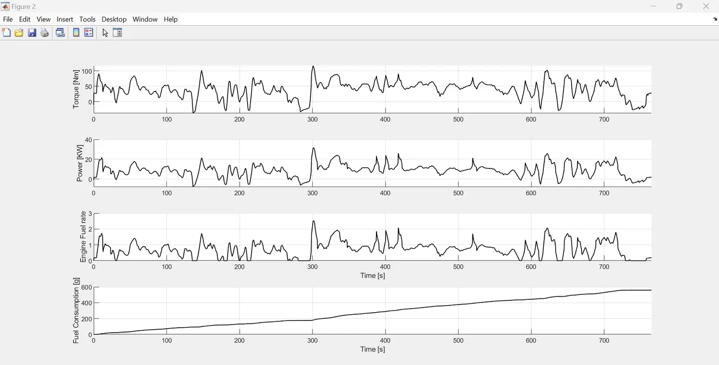
The plots(above) together provide comparative insights into the engine's performance (Torque, power)and fuel consumption behavior over time.

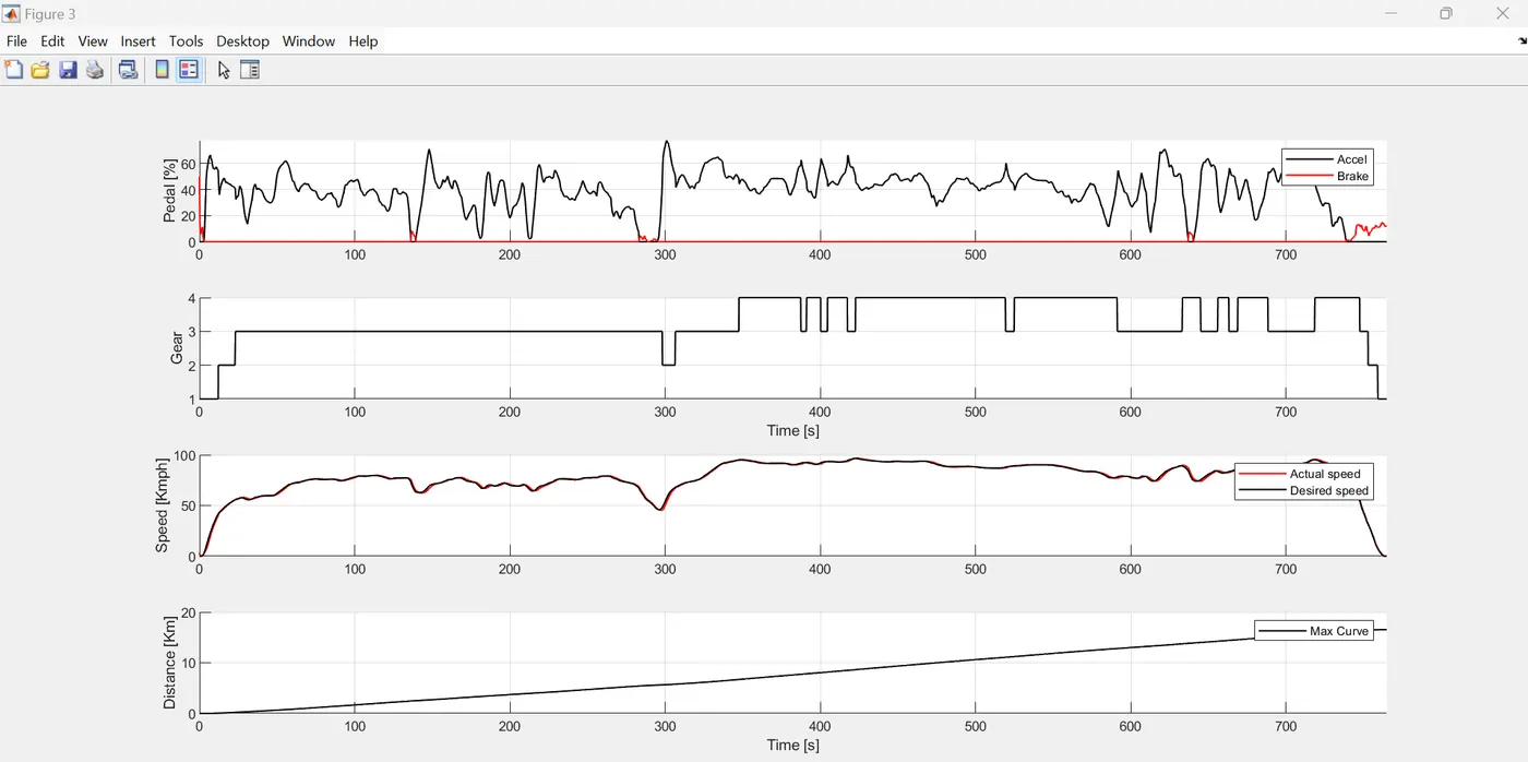
· The vehicle accelerates initially, reaching a desired speed.
· The gear shifts accordingly to maintain optimal performance.
· The actual speed closely follows the desired speed, indicating good control.
· The brake pedal is applied occasionally to maintain or reduce speed as needed.
· The distance travelled increases steadily over time.
· The vehicle stays within the maximum curve speed limit, ensuring safe navigation.

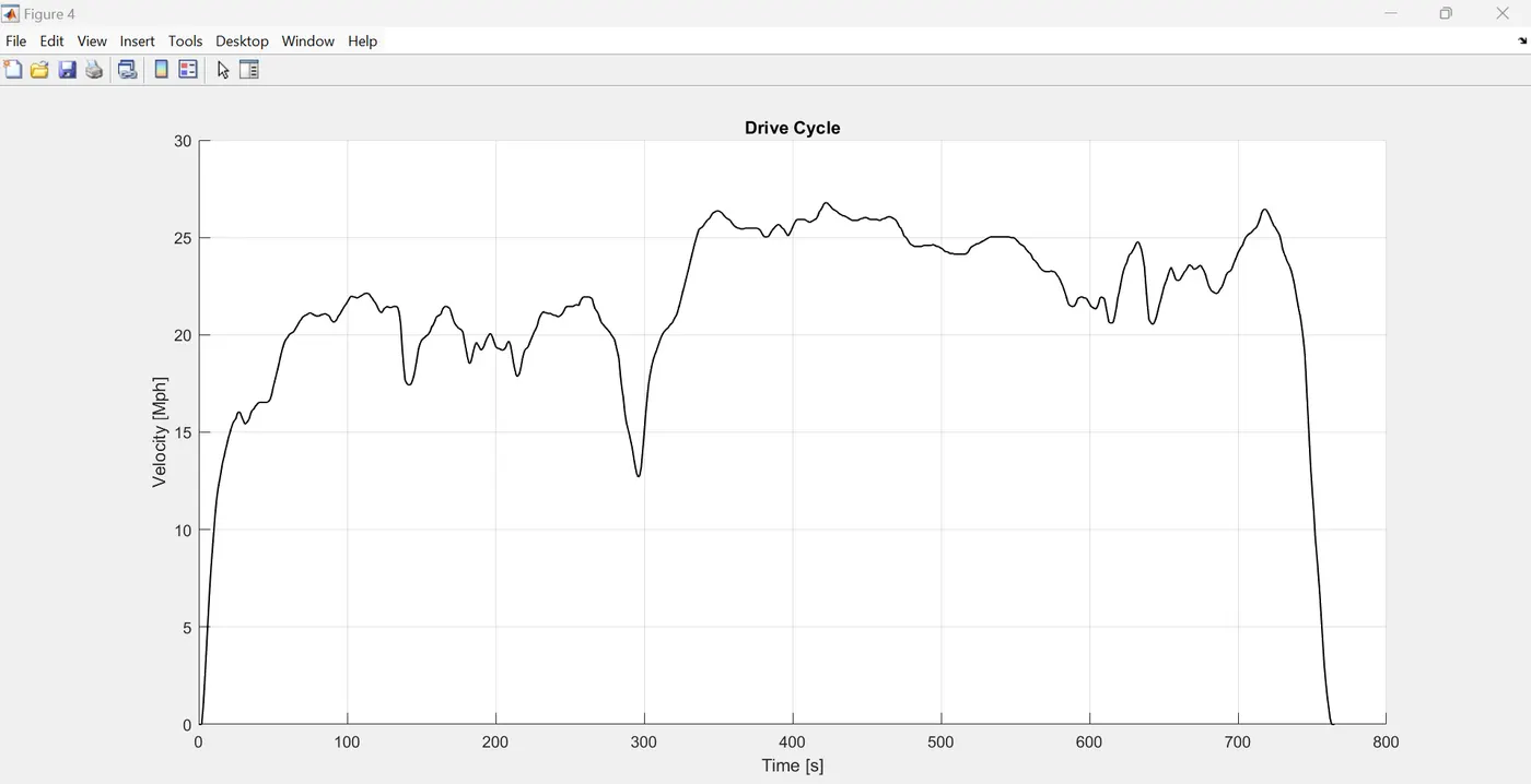
The plot illustrates a representative driving profile that can be used to test the performance and fuel efficiency of a vehicle. The variations in speed mimic real-world driving scenarios, including city driving, highway driving, and acceleration/deceleration events.

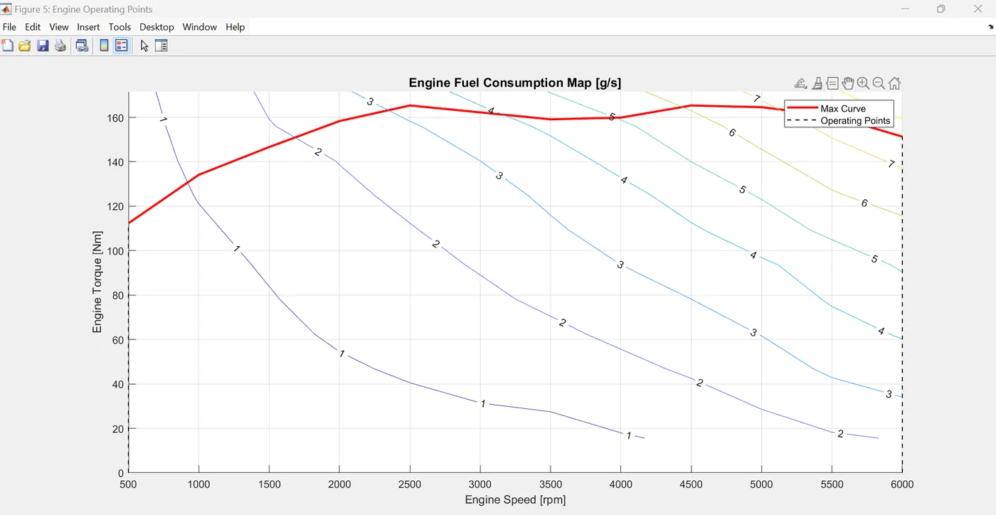
The plot provides insights into the engine's efficiency and fuel consumption characteristics. Here are some key observations:

• Max Curve: The red line shows the maximum torque that the engine can produce at each speed. This line represents the engine's theoretical performance potential.
• Operating Points: The yellow dots indicate the actual operating points of the engine during a specific driving cycle. These points may deviate from the max curve due to factors such as load, throttle position, or gear selection.
• Fuel Consumption: The color contours represent the engine's fuel consumption rate at different operating points. Points closer to the max curve generally have lower fuel consumption rates, indicating more efficient operation.
• Engine Efficiency : The plot highlights regions where the engine operates more efficiently. These regions are typically characterized by lower fuel consumption rates for a given power output.

Conclusion:

This project enables a thorough understanding of vehicle dynamics and fuel consumption modeling, providing essential baseline data for future hybrid vehicle enhancements. The analysis and plots generated will contribute to deeper insights into vehicle performance across different driving conditions.